Highlights

• Cooperative training of two networks that propose an initial segmentation and refine it according to a learned prior, respectively;
• Latent space data augmentation through different masking schemes to train the two networks on challenging and corrupted images and segmentations;
• Study of the method’s usefulness in the context of multi-domain and limited training data.

Introduction

The authors cite multiple motivations for the development of their method:

• Previous segmentations methods that refine initial, rough segmentations require two networks trained separately¹;
• Data augmentation (DA) in the image space requires a lot of expertise to apply, since it can sometimes sacrifice intra-domain performance. Searching for the right kind of DA to apply is also time-consuming.

Methods

The authors name their two networks architecture in reference to behavior science’s model of fast and slow systems of the human brain (often referred to as systems 1 and 2 in the deep learning world). However, this simply boils down to a multi-task encoder-decoder network that performs both segmentation and reconstruction, followed by a segmentation autoencoder, with everything being trained end-to-end.

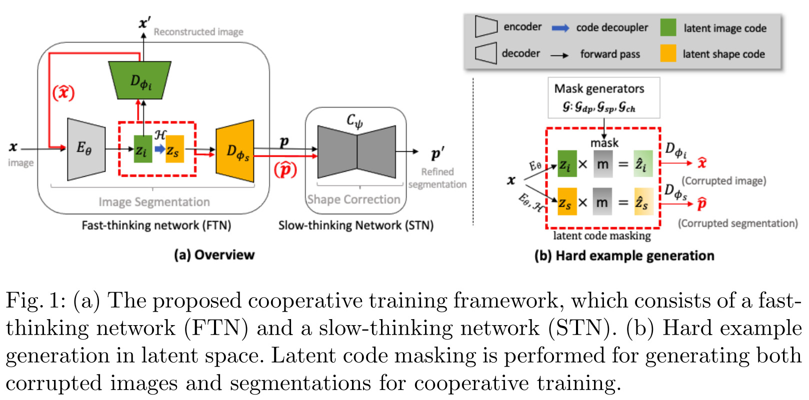
Latent space data augmentation

The authors propose to randomly generate masks to apply to the latent space to drop features and generate corrupted, out of distribution data. In other words, they propose a form of dropout on the latent space vectors.

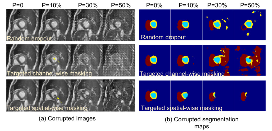
Although not explained directly in the paper, the latent space learned seems to be structured such that \(z \in \mathbb{R}^{c \times h \times w}\). The authors were thus able to use this structure to propose a few different schemes for generating the latent masks.

1. Random Masking with Dropout: Drop random channels from the latent space.
2. Targeted Masking: This scheme seeks to mask the most salient features, which can be determined by using two different methods. First, the gradients on the latent space have to be computed. Afterwards, either the i-th (i) pixels or (ii) channels with the highest mean gradients are masked. In this case, the features are not systemically dropped but rather they are scaled by an annealing factor \(a \in (0,0.5)\).

Cooperative training

By cooperative training, the authors mean that their method is trained on both standard data and data corrupted on-the-fly. Thus, the dual-network is exposed to three hard example pairs, i.e. corrupted images-clean images (\(\hat{x}\), \(x\)), corrupted images-GT (\(\hat{x}\), \(y\)), and corrupted prediction-GT (\(\hat{p}\), \(y\)). The overall loss of the network thus becomes \(\mathcal{L}_{cooperative} = \mathcal{L}_{std} + \mathcal{L}_{hard}\), where \(\mathcal{L}_{hard}\) is defined as:

\[\mathcal{L}_{hard} = \mathbb{E}_{\hat{x},\hat{p},x,y} [ \mathcal{L}_{rec}(\mathcal{D}_{\phi_i}(E_{\theta}(\hat{x})),x) + \mathcal{L}_{seg}(\bar{p},y) + \mathcal{L}_{shp}(\mathcal{C}_{\psi}(\hat{p}),y) + \mathcal{L}_{shp}(\mathcal{C}_{\psi}(\bar{p}),y) ]\]

where

\[\bar{p} = \mathcal{D}_{\phi_i} (\mathcal{H}(E_{\theta}(\hat{x}))), \quad \text{the FTN's predicted segmentation on}~\hat{x}.\]

Data

To test their method, the authors based themselves on the ACDC² and M&Ms³ dataset. The method was trained on 10 patients randomly sampled from ACDC’s training set, and the multi-site M&Ms dataset only served for cross-domain test. The authors also used another 20 patients from the ACDC dataset, which they augmented with different types of MR artifacts to generate challenging intra-domain subsets.

Results

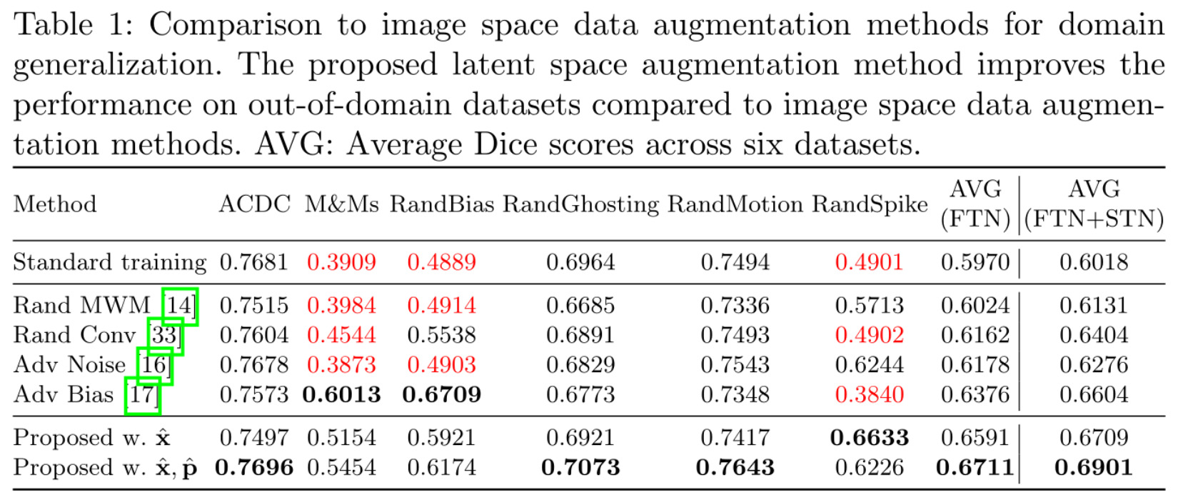
In Table 1, the authors compare their own method with varying degrees of corrupted data (last 2 rows) to SOTA image space DA (middle 4 rows) and a baseline method trained only on the data (1st row). The columns present the performances of each method on different domains, from intra-domain data (ACDC), to cross-domain (M&Ms) and artificially generated challenging domains (Rand*). The last 2 columns compile the average performance of each method on all domains, with or without a refining STN. Note that detailed results shown seem to be for training without a STN only; only average results are available in the case of training with a STN.

References

• Project code repository: https://github.com/cherise215/Cooperative_Training_and_Latent_Space_Data_Augmentation