Highlights

• Closes the gap between the theory and practice on distributional reinforcement learning
• Achieves state-of-the-art results of the Atari 2600 suite of games

Introduction

Distributional Reinforcement Learning (distributional RL) has been proposed as an alternative to standard reinforcement learning where the whole distribution of future rewards is learned instead of its expectation:

\[Z(x,a) \stackrel{D}{=} R(x,a) + \gamma Z(X', A'),\]

where \(Z(x,a) \in \mathbb{R}^{\vert A \vert \times N}\) a set of atoms forming the probability mass function (PMF) of the return distribution. In distributional RL, the goal is to minimize the distance between \(Z_\theta(x,a)\) and \(R(x,a) + \gamma Z_\theta(X',A')\). The Wasserstein metric was proposed to act as a distance metric between the two distributions, but it could not in practice be used as a loss function to be minimized by stochastic gradient descent. The authors instead defaulted to use the KL-divergence between the two distributions with a few unwieldy projection steps to ensure the two distributions shared the same support.

In this work, the authors are able to use the Wasserstein distance as a distance metric by reformulating \(Z\) to model the quantile function of the return distribution instead of its PMF.

Methods

The Wasserstein distance

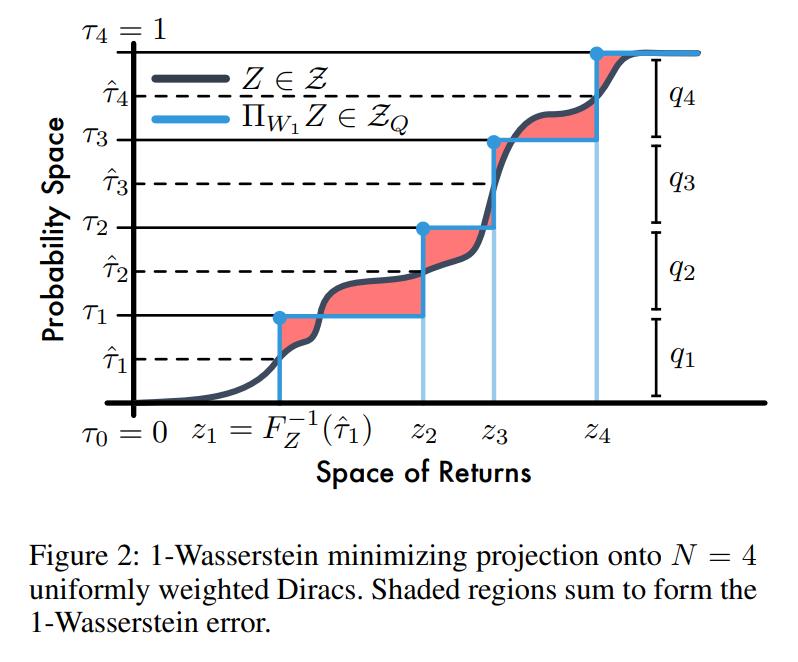
The \(p\)-Wasserstein distance \(d_p\) is the \(L^p\) metric on inverse cumulative distribution functions (inverse CDFs) \(F^{-1}\) between two distribution functions \(U\) and \(Y\):

\[\begin{aligned} d_p(U,Y) &= \Big(\int_0^1 \vert F^{-1}_Y(\omega) - F^{-1}_U(\omega) \vert^p d\omega \Big)^{\frac{1}{p}} \\ F^{-1}_Y(w) &= \text{inf}\{y \in \mathbb{R}: \omega \leq F_Y(y)\} \; \text{// This is the definition of a quantile.} \\ F_Y(y) &= Pr(Y \leq t) \end{aligned}\]

Figure 2 displays the 1-Wasserstein distance between two CDFs.

QR-DQN

To bridge the gap between theory and practice, the authors reformulate the atoms forming \(Z(X,A)\) to instead be the medians of \(N\) quantiles of the distribution instead of the weights of \(N\) possible values. As such, instead of learning the weights of fixed-value atoms, the authors propose to learn the value of fixed-weight atoms \(z_i\).

Formally, \(Z_\theta\) becomes a quantile distribution defined as

\[Z_\theta(x,a) = \frac{1}{N}\sum_1^N \delta_{\theta_{i}(x,a)},\]

with \(\delta\) a Dirac function.

Compared to the original parametrization, the benefits of a parameterized quantile distribution are threefold. First, (1) we are not restricted to prespecified bounds on the support, or a uniform resolution, potentially leading to significantly more accurate predictions when the range of returns vary greatly across states. This also (2) lets us do away with the unwieldy projection step present in C51, as there are no issues of disjoint supports. Together, these obviate the need for domain knowledge about the bounds of the return distribution when applying the algorithm to new tasks. Finally, (3) this reparametrization allows us to minimize the Wasserstein loss, without suffering from biased gradients, specifically, using quantile regression.

Quantile regression¹ is a method for approximating the quantile function of a distribution. The quantile regression loss \(\mathcal{L}^\tau\) for a quantile \(\tau \in [0, 1]\) is a loss function that penalizes overestimation errors with weight \(\tau\) and underestimation errors with weight \(1-\tau\). It can be minimized by stochastic gradient descent and is defined as

\[\mathcal{L}^\tau(\theta) = \mathbb{E}_{\hat{Z} \sim Z}[{\rho_\tau}(\hat{Z} - \theta)],\]

where \(\rho_{\tau}(u)\) can be defined as

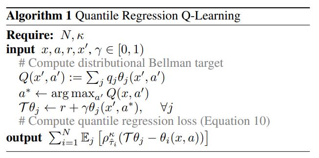
\[\rho_{\tau}(u) = \begin{cases} u(1-\tau) \; &\text{if} \; u < 0 \\ u\tau\; &\text{if} \; u \geq 0 \end{cases}.\]

In practice, the authors use a Huber loss version of the above loss. The authors still base their algorithm on DQN, and the algorithm for the quantile update is given below:

Data

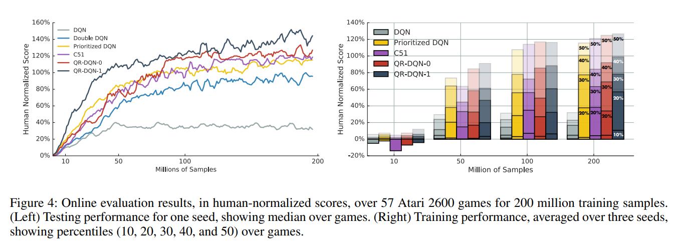
To compare themselves against DQN and C51², the authors used the Arcade Learning Environment.

Results

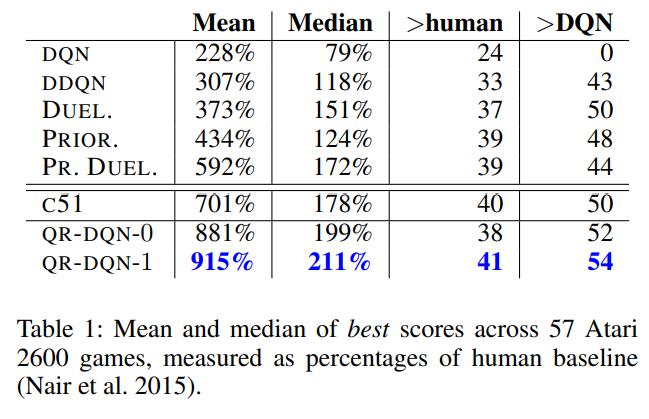
Conclusions

QR-DQN bridges the gap between theory and practice and brings significant performance improvements over C51 and DQN.

References