Highlights

• Proposes a distributional perspective on reinforcement learning
• Achieves state-of-the-art results of the Atari 2600 suite of games

Introduction

Reinforcement learning (RL) typically tries to maximise the expected value (\(Q\)) of the current and future states, as defined by the Bellman Equation:

\[Q(x,a) = \mathbb{E}[R(x,a) + {\gamma}Q(X',A')], x \sim X, a \sim A.\]

¹However, the expectation might not encompass the true distribution of possible returns from a state, for example if one action might lead to disastrous rewards and another to desirable rewards. The expectation, which would fall in the middle, would actually never be encountered by the agent. The authors argue that modelling the full reward distribution allows to keep the potential multimodality of returns in different states, which stabilizes learning and mitigates the effects of learning from a non-stationary policy.

Methods

Theory

Standard reinforcement learning usually minimizes the following distance:

\[\text{dist}(Q_1, Q_2) = \mathbb{E}_{x,a}\Big[\underbrace{(r(x,a) + {\gamma}Q(x',a')}_{Q_2} - \underbrace{Q(x,a)}_{Q_1})^2\Big].\]

From the Bellman equation, the Bellman Operator is defined as

\[\mathcal{T}^\pi Q(x,a) := \mathbb{E}_{x,a,x',a' \sim \pi}[R(x,a) + {\gamma}Q(x',a')],\]

which is a \(\gamma\)-contraction meaning that

\[\lim_{k \rightarrow \infty} (\mathcal{T}^{\pi})^{k}Q = Q_\pi\]

and

\[\text{dist}(\mathcal{T}Q_1,\mathcal{T}Q_2) \leq \gamma \text{dist}(Q_1,Q_2).\]

The authors instead propose to learn policies according to the distributional Bellman Equation, defined as

\[Z(x,a) \stackrel{D}{=} R(x,a) + \gamma Z(X', A'),\]

with

\[Q(x,a) = \mathbb{E}[Z(X,A)]\]

and

\[a^* = \argmax_{a'}Q(x',a').\]

This last line reinforces that the policy still tries to maximize \(Q\), e.g. the expected return. However, the authors propose to learn the full distribution of possible returns, instead of just the expectation.

As such, we will want to minimize the distributional error

\[\sup_{x,a} \text{dist}(R(x,a) + {\gamma}Z(x',a'), Z(x,a)).\]

To do so, there needs to be a Distributional Bellman Operator \(\mathcal{T}_D^\pi\)

\[\mathcal{T}_D^\pi Z(x,a) := \mathbb{E}_{x,a,x',a' \sim \pi}[R(s,a) + \gamma Z(x',a')]\]

which is a \(\gamma\)-contraction s.t.

\[\text{dist}({\mathcal{T}_D}Z_1,{\mathcal{T}_D}Z_2) \leq \gamma \text{dist}(Z_1,Z_2).\]

Finding a distance metric in which \(\mathcal{T}_D\) is a \(\gamma\)-contraction is the main question of the first part of the paper.

For two distributions \(p\) and \(q\) with the same support, the Kullback-Liebler (KL) divergence (in the discrete case) corresponds to

\[KL(p||q) = \sum_{i=1}^N p(x_i)\log \frac{p(x_i)}{q(x_i)}.\]

The KL divergence is simple and appealing and we would hope that \(\mathcal{T}_D\) is a \(\gamma\)-contraction in KL. However, the authors argue that since the predicted and target distributions do not share the same support, the KL divergence would provide an infinite distance between the predicted and target distributions and therefore cannot be used in the current context.

Instead, the authors suggest that the Wasserstein metric can be used instead, and that \(\mathcal{T}_D\) is a \(\gamma\)-contraction in \(\bar{d}_p\).

Even so, it turns turns out that this only holds in the policy evaluation phase (e.g. with fixed policies) and that the control phase (e.g. with the policy improving) remains unsolved.²

Practice

The authors base their work on DQN³. However, instead of having \(Q_\theta\) predict the expected return, the authors propose to learn

\[Z_\theta(x,a) = z_i \; \forall i, \; p_{z_i}(x,a) = \frac{e^{\theta_{i}(x,a)}}{\sum_j e^{\theta_{j}(x,a)}}\]

with

\[z_i = R_\text{min} + i{\Delta}z : 0 \leq i < N, \\ {\Delta}z = \frac{R_\text{max} - R_\text{min}}{N - 1}, \\ R(x,a) \in [R_\text{min}, R_\text{max}].\]

Essentially, \(Z_\theta(x,a)\) predicts a probability mass function (pmf) over the reward domain at \((x,a)\), and \(z_{0..N}\) are the equidistant atoms forming the pmf. This effectively turns \(Z(x,a)\) into a classification problem, allowing us to use standard cross-entropy. We can then use the replay buffer \(D\) of DQN to sample tuples \((x,a,r,x')\) to estimate the target distribution \(r + {\gamma}Z(x', a^*)\) and move \(Z(x,a)\) towards it.

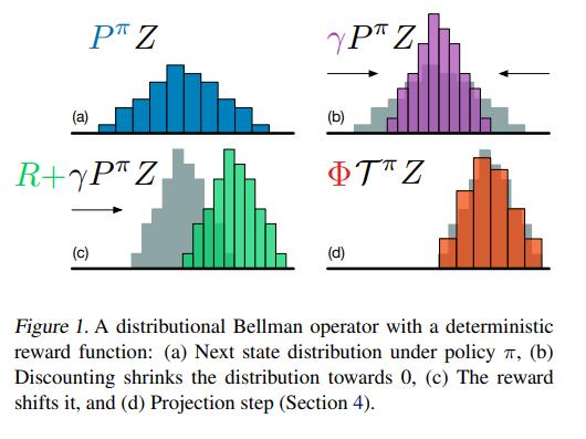
However, \(r + {\gamma}Z(x', a^*)\) shifts the distribution and causes the “target” atoms to be misaligned with the predicted pmf. As such, the authors propose a projection \(\Phi\) to linearly interpolate the target atoms with their neighbors in \(Z_\theta\). Formally, the projected Bellman update is defined as

\[\Phi\hat{\mathcal{T}}Z_\theta(x,a)_i = \sum_{j=0}^N \Big[1 - \frac{\vert{[r + \gamma z_j]_{R_\text{min}^{R_\text{max}}} - z_i}\vert}{\Delta z} \Big]_0^1 p_j(x',\pi(x')).\]

The process is illustrated below.

Then, the standard cross-entropy term of the KL divergence can be used as a loss function

\[\mathcal{L}(x,a) = D_{KL}(\Phi\hat{\mathcal{T}}Z_\theta(x,a) || Z_\theta(x,a)) = \sum_{i = 0}^{N-1} m_i \log z_i(x,a),\]

with \(m_{0...N}\) the projected atoms, which can readily be minimized using gradient descent. The update algorithm is defined below

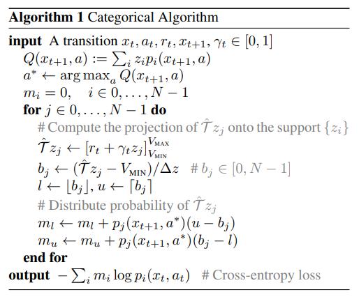
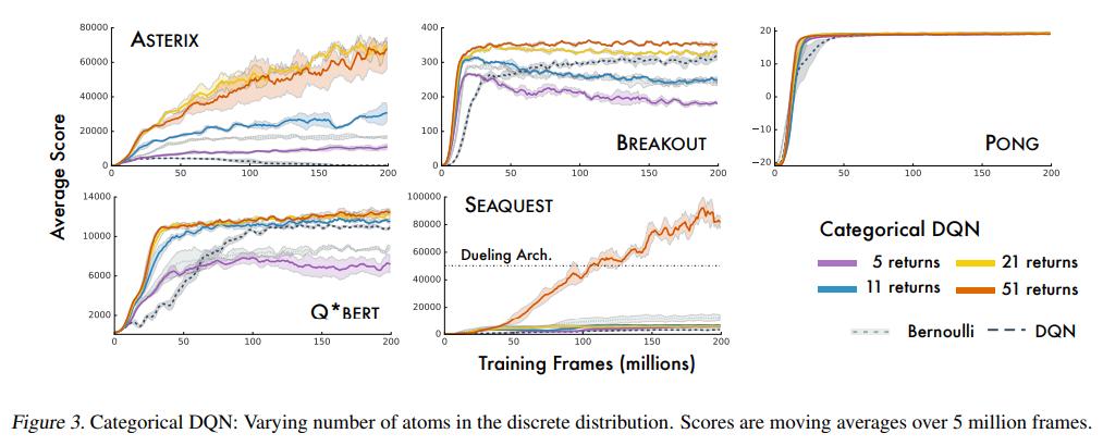
The authors empirically found that 51 atoms worked best, leading to the algorithm’s name: C51.

Data

To compare themselves against DQN, the authors used the Arcade Learning Environment (ALE)⁴.

Results

Varying the number of atoms

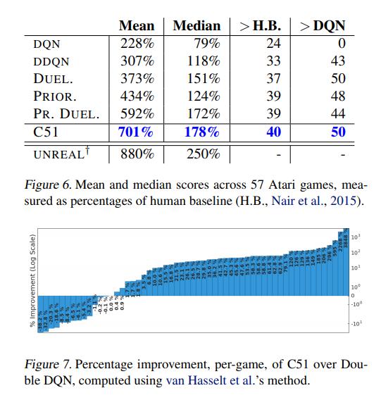
Comparison against (D)DQN

Conclusions

C51 brings significant improvements over DQN.

Remarks

• Several state-of-the-art results have since then used C51 instead of standard DQN to push the benchmark further on Atari 2600, including Rainbow⁵, NGU⁶ and Agent57⁷.

References

• https://mtomassoli.github.io/2017/12/08/distributional_rl/ is a clear explanation of the article and more.