Highlights

• New encoder-decoder architecture that disentangles salient information in images and attributes directly in the latent space;
• At test-time, using continuous attribute values allows to adjust how much of an attribute is perceivable in the generated image.

Introduction

The authors’ goal is to control some attributes of interest in images, for which transformations are ill-defined and training is unsupervised, i.e. where no images with the same content but different values of attributes are available. They achieve this by learning a latent space that is invariant to the attributes of interest, which can then simply be concatenated to any latent vector during the generative process.

Methods

The attribute-invariance is obtained through a process similar to domain-adversarial training, where a classifier learns to predict attributes \(y\) from the latent representation \(z\), while the encoder-decoder tries to simultaneously reconstruct the input and fool the classifier (c.f. Figure 2).

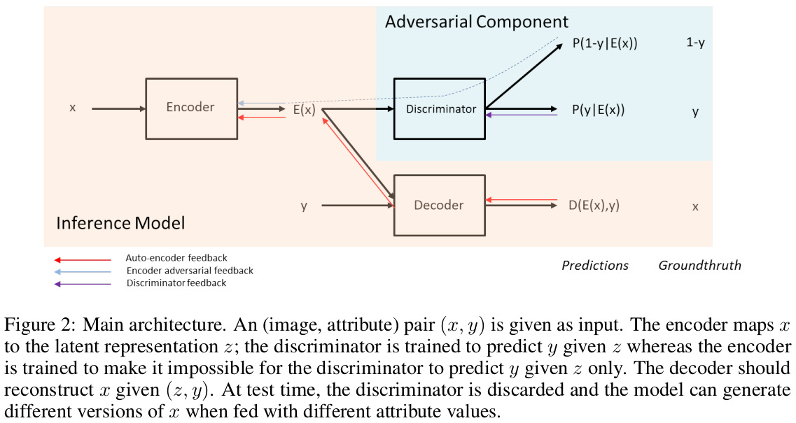
Discriminator objective

The discriminator tries to predict the attributes of the input image given its latent representation according to:

\[\mathcal{L}_{\text{dis}}(\theta_{\text{dis}}|\theta_{\text{enc}}) = -\frac{1}{m} \sum_{(x,y) \in D} \text{log} P_{\theta_{\text{dis}}}(y | E_{\theta{\text{enc}}}(x))\]

Adversarial objective

The encoder tries to learn a latent space that optimizes the two objectives mentioned above: namely a good reconstruction but a bad accuracy from the discriminator:

\[\mathcal{L}(\theta_{\text{enc}},\theta_{\text{dec}}|\theta_{\text{dis}}) = \frac{1}{m} \sum_{(x,y) \in D} \| D_{\theta_{\text{dec}}} (E_{\theta_{\text{enc}}}(x),y) - x \|_{2}^{2} - \lambda_E \text{log} P_{\theta_{\text{dis}}}(1 - y|E_{\theta_{\text{enc}}}(x))\]

Learning algorithm

The overall objective function is:

\[\theta_{\text{dis}}^{(t+1)} = \theta_{\text{dis}}^{(t)} - \eta \nabla_{\theta_{\text{dis}}} \mathcal{L}_{\text{dis}} \big( \theta_{\text{dis}}^{(t)}|\theta_{\text{enc}}^{(t+1)},x^{(t)},y^{(t)} \big) \\ [\theta_{\text{enc}}^{(t+1)},\theta_{\text{dec}}^{(t+1)}] = [\theta_{\text{enc}}^{(t)},\theta_{\text{dec}}^{(t)}] - \eta \nabla_{\theta_{\text{enc}},\theta_{\text{dec}}} \mathcal{L} \big( \theta_{\text{enc}}^{(t)},\theta_{\text{dec}}^{(t)}|\theta_{\text{dis}}^{(t+1)},x^{(t)},y^{(t)} \big)\]

Data

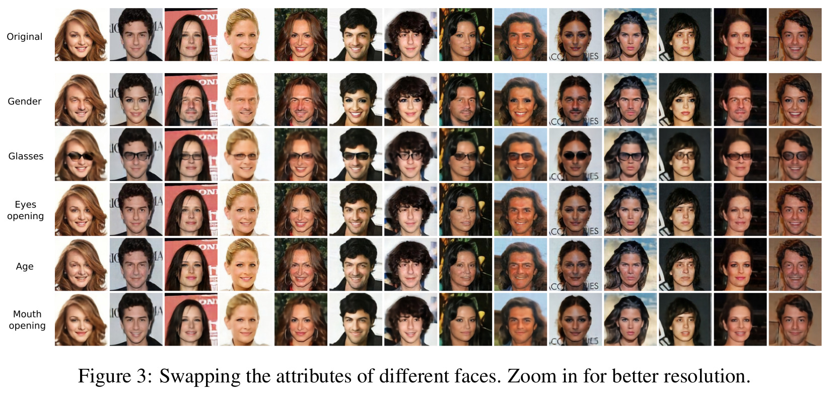
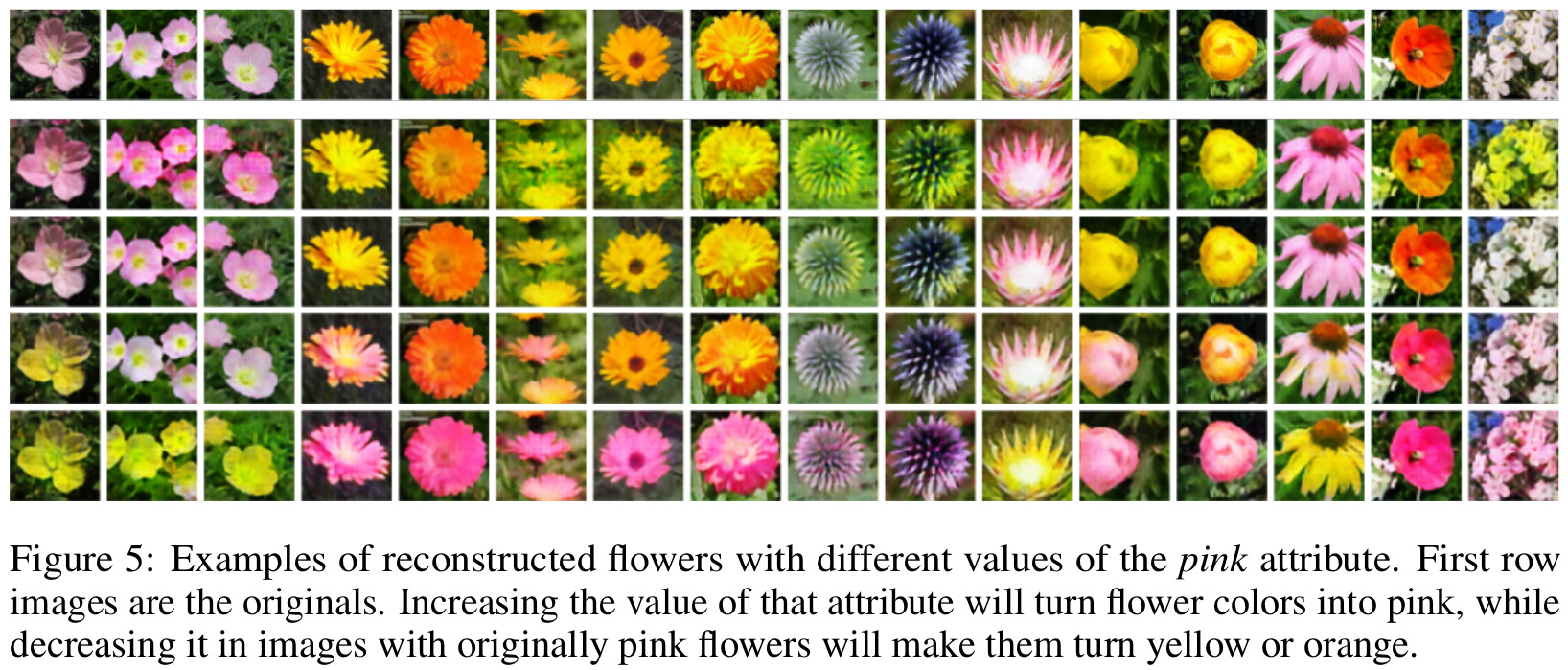
The authors tested the Fader networks mostly on the celebA dataset. They also report some results on the Oxford-102 dataset, which contains images of flowers from 102 categories, but for which the authors added, and used as attribute, the color of the flower.

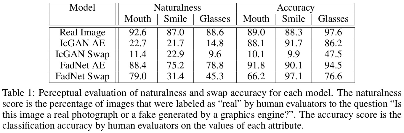
Of note, Mechanical Turk were employed for the quantitative evaluation of the results on the celebA dataset.

Results

Remarks

• In theory, Fader networks should be able to handle continuous data attributes by switching the target of the adversarial component, and adapting its loss from cross-entropy to some kind of regression loss (e.g. MAE, MSE, etc.). However, in practice, the method is known to perform poorly on non-categorical data attribute¹.

• In practice, the addition of an adversarial network makes the training much less stable, as could be expected. Thus, the authors describe (common) implementation details that they required for their method to work, e.g. dropout, discriminator cost scheduling, etc.

References