Highlights

• Decomposition of the variational lower bound that explains the success of \(\beta\)-VAE in learning disentangled representations
• Simple method based on weighted minibatches to estimate the aggregate posterior without additional hyperparameters (the aggregate posterior is required to weight specific terms in the decomposition of the ELBO)
• New \(\beta\)-TCVAE (Total Correlation Variational Autoencoder), which can be used as a plug-in replacement for the \(\beta\)-VAE (and VAE for that matter)
• New information-theoretic disentanglement metric, which is classifier-free and generalizable

Introduction

The paper was written independently from a similar paper by Kim et Mnih¹, and in the same vein propose a tweak on the \(\beta\)-VAE² to further disentangle the learned representation without sacrificing the reconstruction, although the modifications proposed by both papers differ.

Let’s recall the objective of the \(\beta\)-VAE:

\[\tag{1} \mathcal{L}_{\beta} = \frac{1}{N} \sum_{n=1}^{N} (\mathbb{E}_{q} [\log p(x_{n}|z)] - \beta KL(q(z|x_{n})~\|~p(z)))\]

where \(\beta \gt 1\) to encourage disentanglement. This is a more general formulation of the VAE, since we can obtain the original VAE objective by setting \(\beta = 1\) in eq. 1.

Methods

ELBO TC-Decomposition

Let’s define \(q(z|n) = q(z|x_{n})\) and \(q(z,n) = q(z|n) p(n) = q(z|n) \frac{1}{N}\). The aggregate posterior is expressed as \(q(z) = \sum_{n=1}^{N} q(z|n) p(n)\). The authors decompose the KL term like follows:

\[\begin{aligned} \tag{2} \mathbb{E}_{p(n)} [KL(q(z|n)~\|~p(z))] = & \underbrace{KL(q(z,n)~\|~q(z) p(n))}_{\text{1. Index-Code MI}} + \underbrace{KL(q(z)~\|~\prod_{j} q(z_{j}))}_{\text{2. Total Correlation}} \\ & + \underbrace{\sum_{j} KL(q(z_{j})~\|~p(z_{j}))}_{\text{3. Dimension-wise KL}} \end{aligned}\]

The authors describe the purpose of each term:

1. The index-code mutual information (MI) is the mutual information \(I_{q}(z;n)\) between the data variable and latent variable;
2. The total correlation (TC) is a generalization of mutual information to more than two random variables. A heavier penalty on this term is what encourages a disentangled representation;
3. The dimension-wise KL prevents individual latent dimensions from deviating too far from their priors.

Training with Minibatch-Weighted Sampling

The decomposed expression from eq. 2 requires to evaluate the aggregate posterior, which depends on the entire dataset and should thus not be computed during training. This is where Kim and Mnih¹ used the density-ratio trick with a discriminator. Here, the authors propose a weighted version of a naïve Monte Carlo approximation, which they argue doesn’t require hyperparameters or inner optimization loops, to estimate the aggregate posterior.

Let \(\{n_1, \dots, n_M\}\) be a minibatch of samples, their estimator is:

\[\mathbb{E}_{q(z)}[\log q(z)] \approx \frac{1}{M} \sum_{i=1}^{M} \Bigg[\log \frac{1}{N~M} \sum_{j=1}^{M} q(z(n_{i})|n_{j})\Bigg]\]

where \(z(n_{i})\) is a sample from \(q(z \vert n_{i})\) .

\(\beta\)-TCVAE

The proposed \(\beta\)-TCVAE is simply assigning different weights to each of the terms in the ELBO TC-Decomposition:

\[\mathcal{L}_{\beta - TC} = \mathbb{E}_{q(z|n) p(n)} [\log p(n|z) - \alpha I_{q}(z;n) - \beta KL(q(z)~\|~\prod_{j} q(z_{j})) - \gamma \sum_{j} KL (q(z_{j})~\|~p(z_{j}))]\]

Through an ablation study, the authors claim that \(\alpha\) and \(\gamma\) don’t matter much in the results (they were set as \(\alpha = \gamma = 1\) in the end), and that most improvements come from optimizing for \(\beta\) (although they mention this behavior might be specific for each data set).

Mutual Information Gap (MIG)

In order to compare the disentanglement performance of different methods, the authors also propose a parameter-free metric, whereas competing metrics from Higgins et al² and Kim and Mnih¹ both use a classifier.

The authors first propose an empirical mutual information (noted \(I_{n}(z_{j};v_{k})\)) and detailed in the paper) that measures the mutual information between latent variables (\(z_{j}\)) and underlying factors of the generative process (\(v_{k}\)). Based on that measure, they present the full mutual information gap (MIG):

\[\frac{1}{K} \sum_{k=1}^{K} \frac{1}{H(v_{k})} \Bigg(I_{n}(z_{j^{(k)}};v_{k}) - \max_{j \neq j^{(k)}} I_{n}(z_{j};v_{k})\Bigg)\]

where \(j^{(k)} = \argmax_{j} I_{n}(z_{j};v_{k})\) and \(K\)s are the factors of the generative process. The division by \(H(v_{k})\) (bound of the empirical mutual information) ensures that MIG is bounded by 0 and 1.

Data

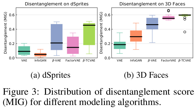
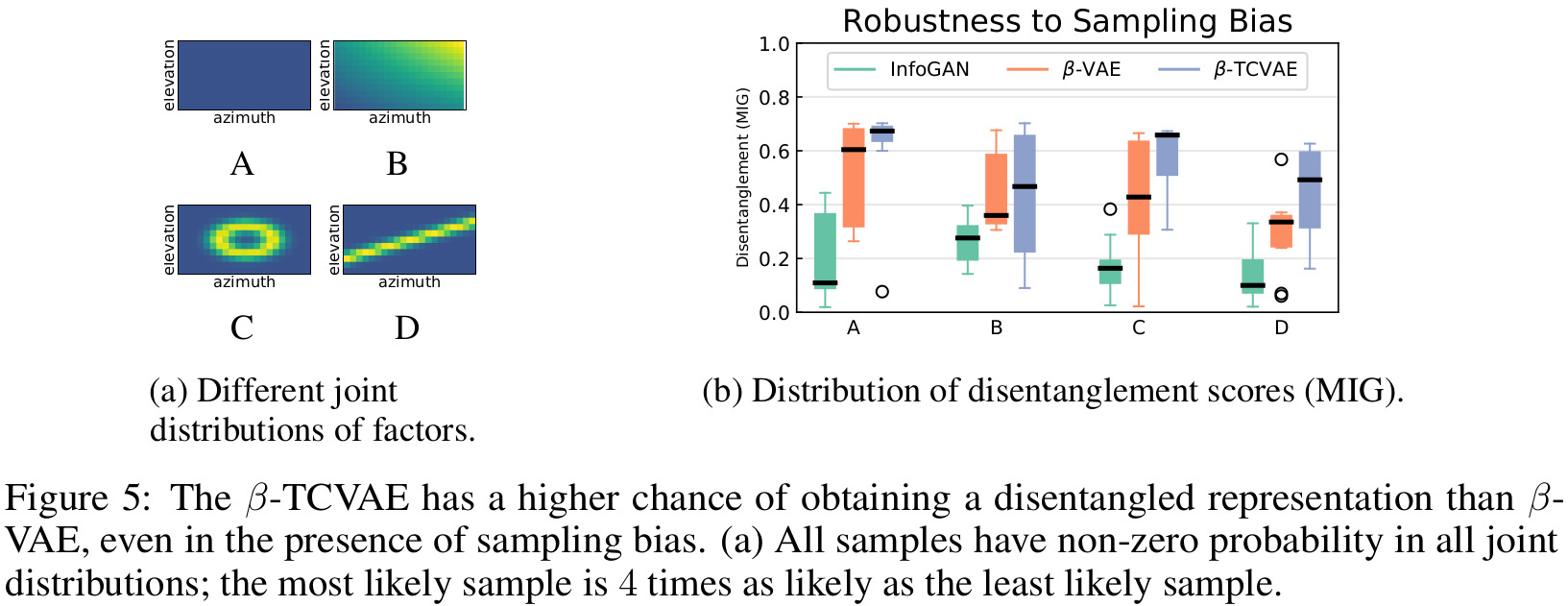
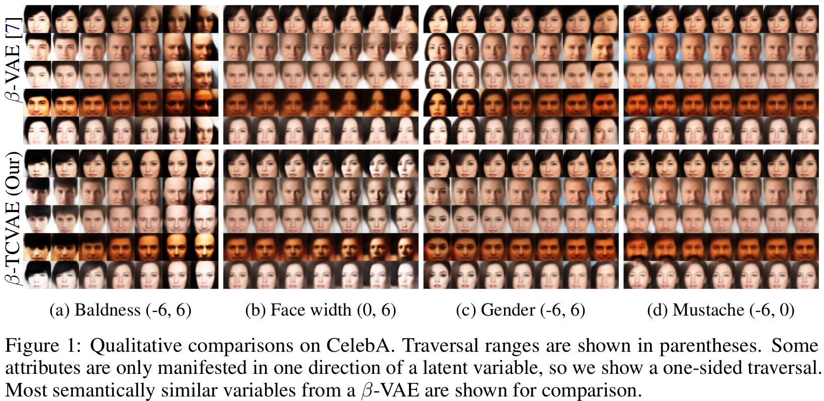
Experiments were performed on two data sets with known generative factors (dSprites and 3D Faces) and one unsupervised data set (CelebA).

Results

References