Introduction

This post is a review of uncertainty estimation methods with an emphasis on classification and segmentation.

Evaluating Uncertainty

Model calibration

A neural network trained for classification is said to be calibrated if its confidence is equal to the probability of it being correct. For example, given 100 predictions with an average confidence of 0.7, 70 predictions should be correct. This can be expressed :

\[\mathbb{P} ( \hat{Y} = Y | \hat{P} = P ) = p \quad \forall p \in [0, 1]\]

where \(\hat{Y}\) is the predicted class and \(\hat{P}\) is the predicted probability.

Calibration is often shown with reliability diagrams ¹ (see figures in the following sections). These diagrams are built by splitting the samples into bins according to their confidence. The accuracy for each bin each calculated and should correspond to the average confidence. The difference between the accuracy and confidence is known as the gap. Averaging the gap for all bins gives the expected calibration error (ECE) ².

Uncertainty-error overlap

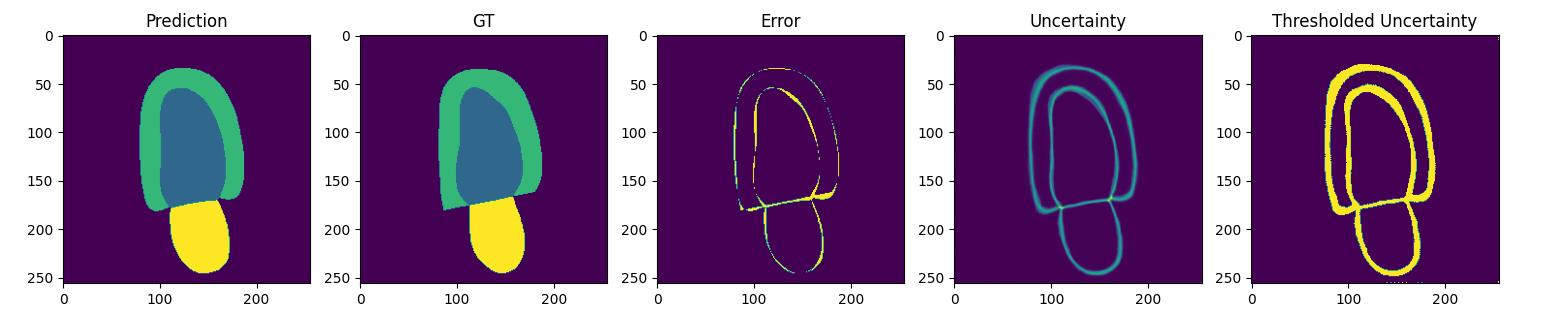
In the case of segmentation, the uncertainty of a prediction can be predicted via an uncertainty map. An uncertainty map is an uncertainty prediction for each pixel. Uncertainty map quality can be evaluated by computing the uncertainty-error overlap. Uncertainty-error overlap is computed by obtaining the dice score of the uncertainty map and a pixel-wise error map between the prediction and the groundtruth segmentation map. The following figure illustrates the uncertainty map and error map for a given sample from the Camus dataset ³.

Uncertainty Estimation Methods

Softmax

The simplest way to estimate uncertainty for a classification task is to use the probabilities of the softmax output layer. Given a vector \(\vec{p}\) of probabilities produced by a softmax operation with \(C\) classes, one can evaluate the uncertainty by computing:

• The maximum class probability: \(max(\vec{p})\). The value must be flipped to obtain uncertainty as most certain samples will have high confidence.
• The margin between the top 2 classes: \(sort(\vec{p})_0 - sort(\vec{p})_1\). The value must be flipped to obtain uncertainty because the smaller the difference between the two most probable classes, the higher the uncertainty.
• The entropy of the vector: \(\sum_{i=0}^C \vec{p}_i \log(\vec{p}_i)\). The higher the entropy, the higher the uncertainty as the entropy will be at its highest if all classes are equally probable \(\vec{p}_i = \frac{1}{C}\).

In the case of a simple classification output, this results in one uncertainty value per classification. In the case of segmentation, the uncertainty evaluation is done for each pixel and results in an uncertainty map with one real value per pixel.

Temperature Scaling

Guo et al. ⁴ show that neural networks, especially deep networks, tend to be miscalibrated as can be seen in the following reliability diagrams.

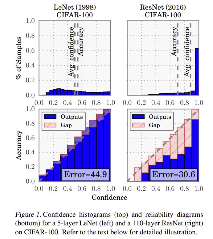
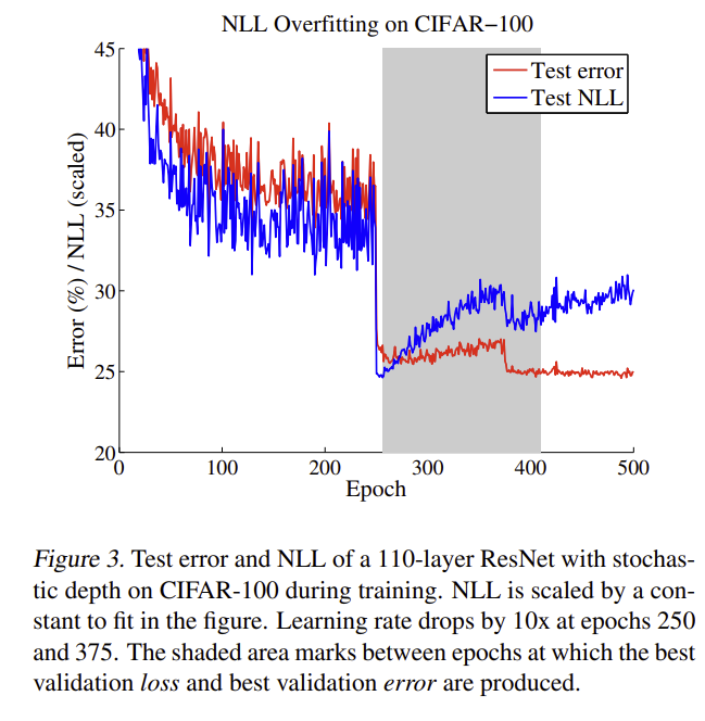
They show that this is because neural networks can overfit on the negative log-likelihood loss while the classification error rate stays constant.

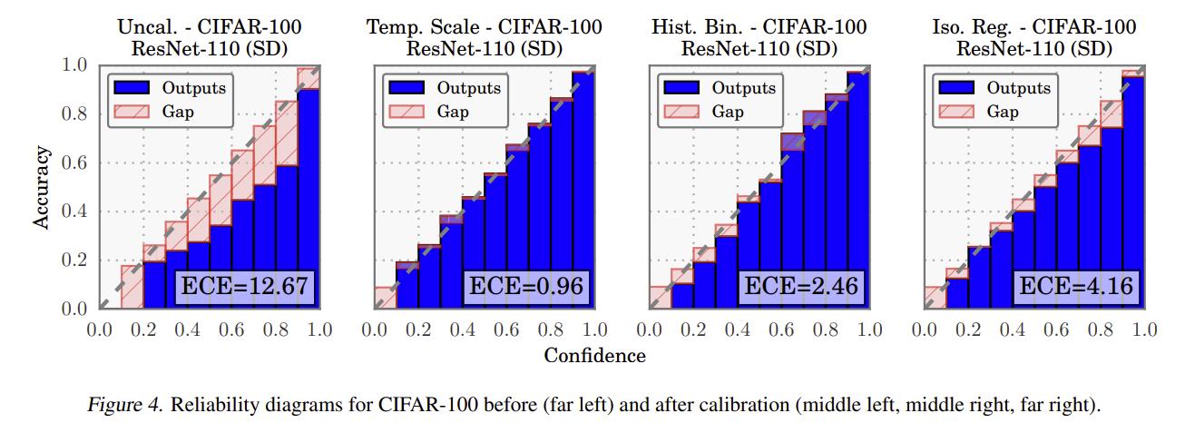
They propose temperature scaling as a post-processing step to solve the issue. This operation adds a learned parameter \(T\) that is trained to minimize the negative log-likelihood on the validation data once the full training is done. This parameter acts on the softmax in the following way:

\[P(y|x, w) = \frac{e^{f^w(x_i) / T}}{\sum_j e^{f^w(x_j) / T}}\]

The value for \(T\) will not change the classification predictions but learning a high value will lower the confidence of the predicted class and therefore can increase calibration as shown in the following figure.

Ensembles

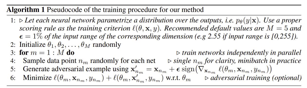
Ensemble of neural networks can be a straightforward way of estimating uncertainty by quantifying the disagreement between each model in the ensemble. Lakshminarayanan et al. propose adding adversarial examples to this training procedure ⁵.

Bayesian Neural Networks

Bayes by Backprob

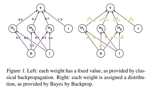
Blundell et al. introduce a way of training Bayesian neural networks known as Bayes by Backprop in Weight Uncertainty in Neural Networks ⁶. Instead of having a point estimate for each weight, Bayesian neural networks learn a distribution over each parameter.

The goal of Bayesian neural networks is to find the posterior distribution of the weights, which can be expressed with Baye’s theorem:

\[P(w|D) = \frac{P(D|w)P(w)}{P(D)}\]

Given this distribution and a new sample \(x^*\), we can get a predictive distribution for \(y^*\):

\[P(y^*|x^*, D) = \int P(y^* | x^*, w) P(w|D) dw\]

However, there is no tractable analytical solution for \(P(w|D)\) for neural networks. Variational inference is therefore used to estimate the true posterior with a variational approximation \(q(w|\theta)\). This gives the following loss function:

\[\theta^* = \argmin_\theta KL[ q(w|\theta) || P(w|D) ]\] \[\theta^* = \argmin_\theta \int q(w|\theta) \log \frac{q(w|\theta)}{P(w)P(w|D)}\] \[\theta^* = \argmin_\theta KL[ q(w|\theta) || P(w) ] - \mathbb{E}_q(w|\theta)[\log P(w|D)]\]

MC Dropout

Training Bayesian neural networks is not trivial and requires substantial changes to the training procedure. Gal et al. show that neural networks with dropout can be used as an approximation for Bayesian nets ⁷. By using dropout at test time, one can generate a Monte Carlo distribution of predictions which can be used to estimate the uncertainty of the prediction.

What uncertainties are needed?

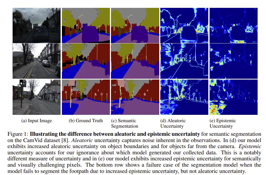
Kendall et al. describe two types of uncertainty in What Uncertainties Do We Need in Bayesian Deep Learning for Computer Vision? ⁸. Firstly, epistemic uncertainty is the uncertainty in the model weights. This can be represented with Bayesian nets or MC dropout. This type of uncertainty can be decreased with more data. The second type of uncertainty is aleatoric uncertainty; the uncertainty in the data. This type of uncertainty cannot be reduced by more data as it is inherent to the data. Aleatoric uncertainty can be homoscedastic (constant for all inputs) or heteroscedastic (dependant on the input sample).

As mentioned estimating epistemic uncertainty can be done using MC dropout. The prediction is given by:

\[p(y=c| x, D) \approx \frac{1}{T} \sum_{i=1}^T Softmax(f^{w^T}(x))\]

where \(T\) is the number of Monte Carlo iterations and \(w^T \sim q(w|\theta)\) with \(q(w|\theta)\) being the dropout distribution. The epistemic uncertainty is obtained by computing the entropy of the resulting probability vector.

Estimating heteroscedastic aleatoric uncertainty involves predicting the variance. Predicting variance is easier to understand in the case of regression. Given a Gaussian assumption, the standard mean squared error loss function is the following:

\[L(\theta) = \frac{1}{N} \sum_{i=1}^N ||y_i - f^w(x_i)||^2\]

This is equivalent to predicting the mean of the gaussian distribution. However, it is also possible to predict the variance:

\[L(\theta) = \frac{1}{N} \sum_{i=1}^N \frac{1}{2\sigma^w(x_i)^2} ||y_i - f^w(x_i)||^2 + \frac{1}{2}\sigma^w(x_i)^2\]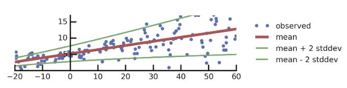

⁹

In the case of classification, the formulation is slightly more complicated. Given a model logits \(f^w(x_i)\) and variance prediction \(\sigma^w(x_i)\), the logits can be corrupted by Gaussian noise with variance \(\sigma^w(x_i)^2\).

\[\hat{x}_i | w \sim \mathcal{N}(f^w(x_i), \sigma^w(x_i)^2)\] \[\hat{p}_i = \text{Softmax}(x_i)\]

The expected log-likelihood is therefore:

\[\log E_{\mathcal{N}(f^w(x_i), \sigma^w(x_i)^2)}[\hat{p}_{i,c}]\]

where \(c\) is the groundtruth class.

In practice, it is not possible to integrate the Gaussian distribution analytically. A Monte Carlo approximation must be done to sample from the distribution.

They show their results on the cityscape dataset:

Auxiliary networks

Many papers use auxiliary networks to estimate uncertainty. Here are a few examples:

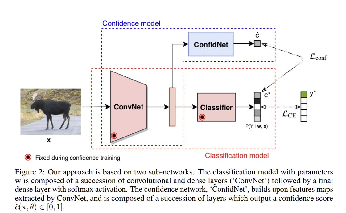
Corbière et al. propose using the True Class Probability (TCP) instead of using the maximum class probability to estimate confidence ¹⁰. They do this by learning TCP with a second network trained to predict the softmax probability of the groundtruth class generated by a pretrained and frozen classification network.

Further reading

Review articles

The following articles offer reviews of many different methods.

• Assessing Reliability and Challenges of Uncertainty Estimations for Medical Image Segmentation, Jungo et al. 2019.
• Estimating uncertainty in deep learning for reporting confidence to clinicians in medical image segmentation and diseases detection, Ghoshal et al. 2020.
• Leveraging Uncertainty Estimates for Predicting Segmentation Quality, DeVries et al. 2018

Other

• Local Temperature Scaling for Probability Calibration, Ding et al. 2020 (Applying temperature scaling to segmentation)

References