Self-Supervised MultiModal Versatile Networks
Highlights
- Introduce the notion of a MultiModal Versatile (MMV) network, that can ingest multiple modalities and outputs
common representations useful for downstream tasks;
- The paper especially studies how best to combine the modalities, so that the common representations respect properties deemed useful by the authors.
- Introduce the process of deflation, to efficiently apply networks on video data to static images.
Introduction
The authors’ motivation is to propose a network for joint video-audio-text representation that respects four properties:
- Able to take as input any of the three modalities;
- Respect the specificity of the modalities: audio and video are much finer than text, i.e. their dimensionality is higher and they contain a lot of details, by contrast to the high-level, coarse information provided by text data;
- Enable the different modalities to be easily compared even when they are never seen together during training;
- Efficiently applicable to visual data coming in the form of dynamic videos or static images.
Methods
A video \(x\) can be described as a combination \({x_m}\) of different modalities \(m \in M\), e.g. vision \(x_v\), audio \(x_a\) and text \(x_t\). For each modality \(x_m\), the authors propose to learn a specific backbone neural network \(f_m\) that outputs a representation vector of dimension \(d_m\), such that \(f_m: \mathcal{X}_m \rightarrow \mathbb{R}^{d_m}\). Finally, modality specific projection heads \(g_{m \rightarrow s}\) map these representation vectors to vectors \(z_{m,s}\) in a space \(S_s\) shared between a set of modalities \(s\) (e.g. \(s = va\) for a joint visual-audio space). Thus, the final representation of an input modality is:
\[z_{m,s} = g_{m \rightarrow s}( f_m(x_m) )\]The authors’ goal is to find the best way to combine the modality specific representation vectors into a shared space, a process which they represent by what they call embedding graphs. The figure below represents different embedding graphs discussed in the paper:
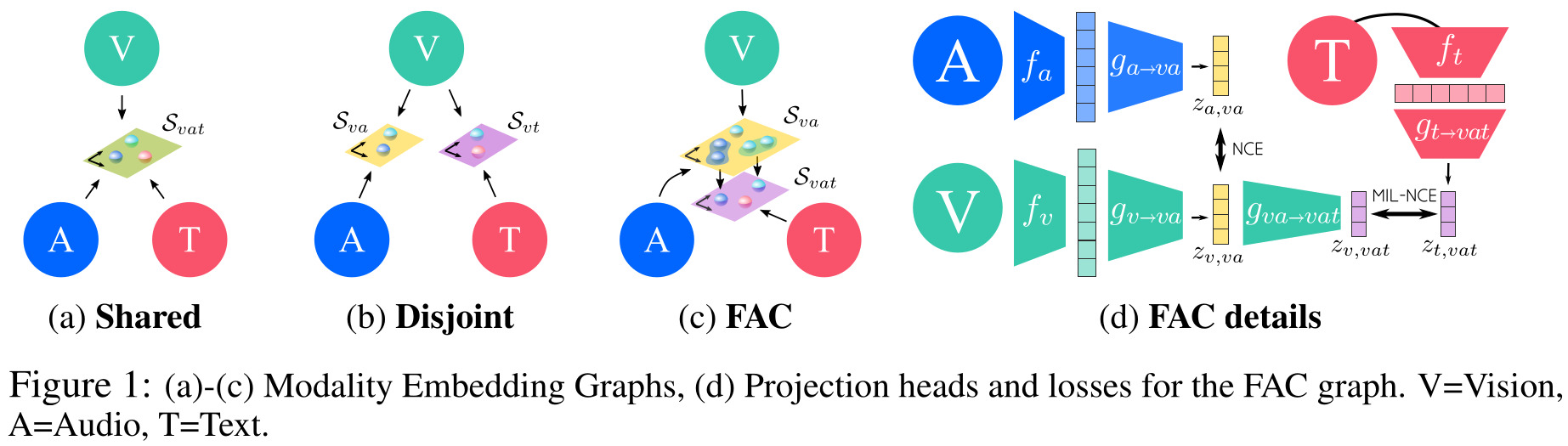
MMV: MultiModal Versatile Networks
Between the different embedding graphs proposed in Fig. 1, the authors settle on the Fine And Coarse spaces (FAC). They argue that a higher-dimensional video-audio shared space (\(S_{va}\)) is necessary, since these modalities contain finer details than the high-level, coarse text modality. However, since another projection head maps \(S_{va}\) to the shared video-audio-text space (\(S_{vat}\)), then ultimately all modalities can still be compared to one another easily.
To train their network in a self-supervised manner, the authors use a contrastive loss in the shared embeddings (e.g. \(S_{va}, S_{vat}\)), where modalities sampled from the same video are considered positive pairs, and modalities sampled from different videos are negative pairs:
\[\mathcal{L}_x = \lambda_{va} \text{NCE}(x_v,x_a) + \text{MIL-NCE}(x_v,x_t)\]where \(\lambda_{mm'}\) is the weight for the modality pair \(m\) and \(m'\).
The authors argue that a variant of the NCE loss, MIL-NCE (from some of the same authors) should be used between video and text, since text is not as closely aligned temporally to video as audio.
Video to image network deflation
The goal is to be able to efficiently use the model trained on videos to process static images, without specifically training or finetuning on static images. A standard trick is to repeat the image to obtain a static video, but the authors claim that there is a more efficient way of doing things.
The idea is to deflate the network to get rid of the temporal dimension. For example, on 3D convolutional networks, this means summing the filters over the temporal dimension. However, the catch is that because of zero-padding at the start/end of the clip, summing the filters will not lead to the same result as processing the static video. Therefore, the solution proposed by the authors is to learn new parameters \(\gamma\) and \(\beta\) in batch normalization layers to correct this boundary effect. \(\gamma\) and \(\beta\) are trained to minimize the \(L_1\) loss between the output of the deflated network on images and the output of the original network given the static video.
Data
The authors train on two datasets:
- HowTo100M: 100 million narrated clips (with text extracted using ASR) coming from 1 million unique videos
- AudioSet: 2 million 10-second sound clips, with corresponding video but missing text
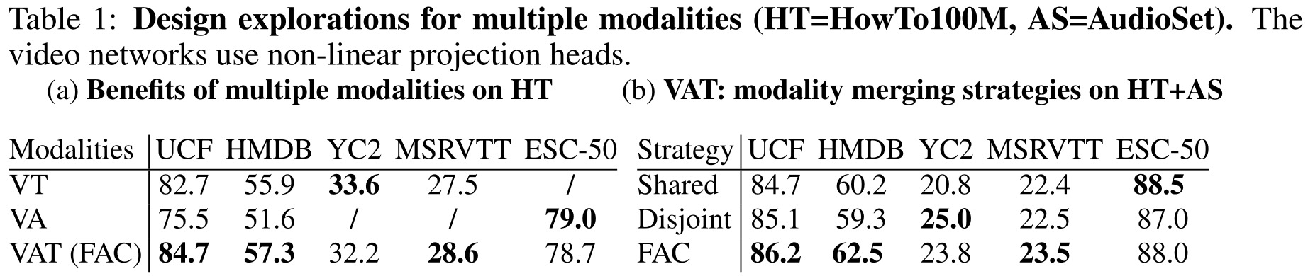
Results
The methods are tested on a variety of downstream tasks by simply learning a linear classifier on top of the modality specific representation vectors \(f_m(x_m)\), with the feature model \(f_m\) either frozen or finetuned:
- Action classification (from video): to evaluate video representation
- Audio classification: to evaluate audio representation
- Zero-shot text-to-video retrieval: to evaluate text-video representation
- Image classification: to evaluate video representation’s transfer to images
Remarks
- The authors insist that they do not learn construct the audio-text shared space explicitly, but rather learn it with the video as intermediary. However, they have two different audio tracks: the narration and the video audio itself. So it seems to me that they could learn explicitly to associate audio and text if they used the video audio. Or are both the video audio and the narration merged into a single audio track?
References
- Code is available on GitHub: https://github.com/deepmind/deepmind-research/tree/master/mmv