Introduction

Finding governing equations for dynamical systems is an essential task in many scientific fields. However, these equations are often unknown. With the increased availability of large datasets for time series data, many data-driven model discovery approaches have been proposed. However, to find interesting models many of these methods required the data to be in specific coordinate systems which is often not the case.

Authors propose a method to discover both the intrinsic coordinates systems and governing equations of high dimensional data using a combination of Auto-encoders and Sparse identification of nonlinear dynamics (SINDy)¹.

Methods

Sparse identification of nonlinear dynamics (SINDy)

The goal of the SINDy algorithm is to find a parsimonious dynamical model from time-series data.

Given snapshot data \(x(t) \in \mathcal{R}^n\), the goal is to find a function \(\mathbb{f}\) that fits a dynamical system

\[\frac{d}{dt} x(t) = \mathbb{f}(x(t))\]

Given \(m\) data samples of length \(n\), data snapshots and derivative snapshots are stacked to create \(X, \dot{X} \in \mathcal{R}^{m \times n}\). This method assumes the snapshot derivatives \(\dot{x}(t)\) are available or can be calculated from the data.

Using a library of \(p\) candidate basis functions \(\Theta(X) = [\theta_1(X), \theta_2(X), ..., \theta_p(X) ]\) (functions such as polynomials and trig. functions), \(\mathbb{f}\) can be approximated.

\[\dot{X} = \Theta(X)\Xi\]

where \(\Xi = (\xi_1, \xi_2, ...\xi_n) \in \mathcal{R}^{p \times n}\) is the set of coefficients for each candidate function.

The goal of this method is to find a parsimonious model by using a sparse regression to find \(\Xi\):

\[min_\Xi ||\dot{X} - \Theta(X)\Xi||_2^2 + \lambda ||\Xi||_1\]

SINDy Autoencoders

SINDy works best with low dimensional data. To work with high dimensional data, such as videos, authors present SINDy Autoencoders, a new method that combines SINDy and autoencoders. Their method leverages the representative learning of autoencoders to discover the coordinate system and SINDy to find the sparse dynamical model in the autoencoder’s latent space.

If the data \(x(t)\) is high dimensional, the goal is to find the function \(\mathcal{g}\):

\[\frac{d}{dt} z(t) = \mathbb{g}(z(t))\]

where \(z(t) = \varphi(x(t)) \in \mathcal{R}^d (d \ll n)\)

SINDy algorithm is applied on the latent variables to find the governing equations in the latent space with appropriate basis functions.

\[\frac{d}{dt} z(t) = \mathbb{g}(x(t)) = \Theta(z(t))\Xi\]

The method is trained with 4 loss terms.

• Reconstruction loss
• SINDy loss in \(\dot{x}\)
• SINDy loss in \(\dot{z}\)
• SINDy regularization

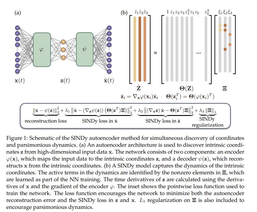
The latent variable time derivatives can be computed by \(\dot{z}(t) = \nabla_x\varphi(x(t))\dot{x}(t)\). (Essentially forward propagation of the derivates of \(x\)).

To achieve a truly sparse model, coefficients in \(\Xi\) under \(0.1\) are set to zero for the remainder of training at every 500 epochs.

Results

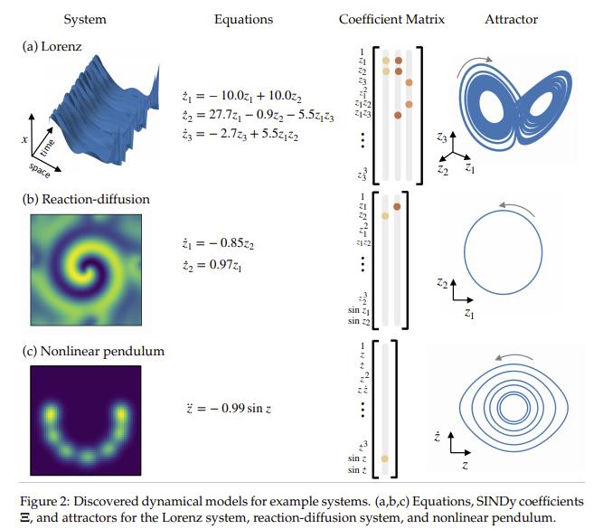
Authors test their method on 3 systems with well know equations. They generate synthetic high dimensional data and train their autoencoder to find the underlying coordinate system and equations.

Chaotic Lorenz system

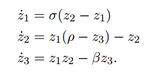
The authors construct a high dimensional example base on the chaotic Lorenz system defined by:

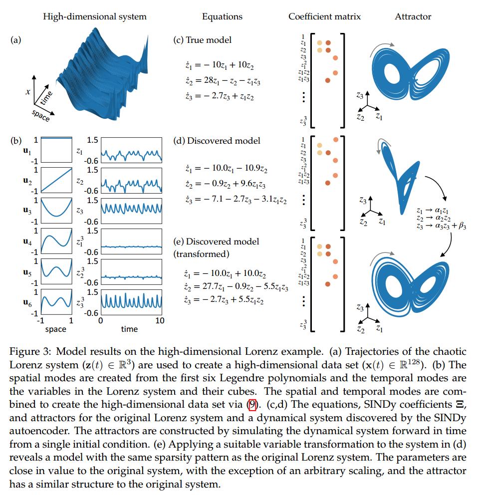
The high dimensional data is created with 6 fixed spatial modes \(u_1,..., u_6 \in \mathcal{R}^{128}\) given by Legendre polynomial:

Their model discovers a correct model and given an affine transformation the authors recover the original model.

Reaction-diffusion

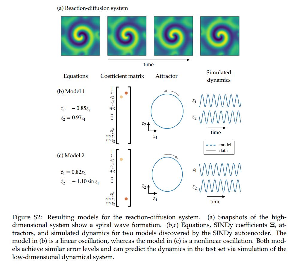
Authors test their method on the lambda-omega reaction-diffusion system and obtain the following results:

Nonlinear pendulum

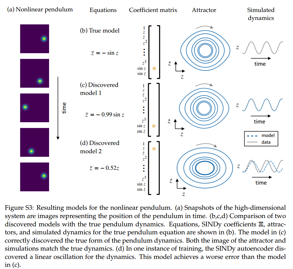
The non-linear pendulum is governed by a second order differential equation:

\[\ddot{z} = - \sin z\]

Authors generate snapshot images with a two dimensional Gaussian centered at the center of mass of the pendulum given by the angle z.

The position of the pendulum can be represented by one variable and therefore the latent dimension is 1. Authors point out that linear autoencoders (such as PCA) could not learn the representation of this data and a non-linear autoencoder was required.
The second order derivatives must be computed for \(x\) and propagated to the latent space.

They obtain the following models:

Conclusions

Authors point out that this method requires approximately noise-free data because their method requires good estimates of the derivatives.

Code is available here: https://github.com/kpchamp/SindyAutoencoders

References