A generative modeling approach for interpreting population-level variability in brain structure
Highlights
- A generative modeling framework, such as a \(\beta\)-VAE in this case, coupled with structured perturbations allows to probe the latent space to provide insightful representations of the brain structure.
Introduction
Disentangling how neural structure varies across individuals is key to better interpret the effects of disease, learning, and aging on the brain. Yet, disentangling the factors that explain such variability remains a challenge. The issue is exacerbated by the large number of features that can be extracted in neuroimaging studies.
Unsupervised data-driven, dimensionality reduction methods can provide ways to identify better the sources of variation across a population. Authors introduce a \(\beta\)-VAE-based framework that allows to interpret brain structure variation in terms of the latent factors.
Methods
Authors base their framework on a \(\beta\)-VAE. A \(\beta\)-VAE is composed of an encoder and a decoder, much like a regular autoencoder,

where \(p(x)\) denotes our dataset’s distribution over the high-dimensional image space, \(q(z \vert x)\) and \(q(x \vert z)\) are the distribution of the estimated encoder and estimated decoder respectively, and \(p(z)\) is the assumed prior on latent variable.
\(\beta\)-VAE introduce a regularization parameter for the KL-divergence term of the model’s loss:

Increasing the value of \(\beta\) encourages a certain degree of clustering, whereas lowering it encourages dispersion of similar elements in the latent space. Thus, an appropriate value of \(\beta\) can allow for disentangling the latent factors to a given extent.
Authors found that an 8-dimensional space and \(\beta = 3\) provided best results in their setting.
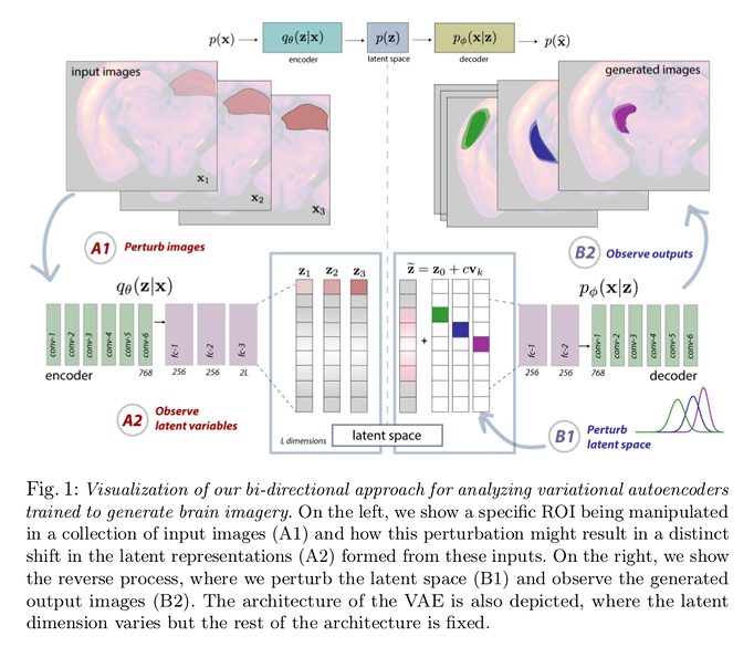
To investigate the interaction between the image space and the \(\beta\)-VAE’s latent space authors performed perturbations on both the input image space and the latent space:
- Map a latent variable’s receptive field, i.e. which pixels in the input space impact each latent factor’s activations. In order to do so, they apply a given localized perturbation to an input image following, \(\widetilde{\mathbf{x}} = \mathbf{x}_{0} + w \mathbf{p}_{\ell}\) where \(\mathbf{x}_{0}\) is the original image, \(\mathbf{p}_{\ell}\) is a region-specific perturbation, and \(w\) is the perturbation weight, and examine the obtained vector’s along its dimensions.
To investigate this aspect, authors applied masks to remove all content from different ROIs, modulated their intensity with perturbation weights \(w\), and fed these perturbed images into the encoder. They then fit a Gaussian to the resulting latent codes across all image examples.
- To investigate a latent variables projective field, i.e. which dimension of the latent variable affects the image space features, authors perform the perturbation according to \(\widetilde{\mathbf{z}} = \mathbf{z}_{0} + c \mathbf{v}_{k}\) where \(\mathbf{z}_{0}\) is the original latent vector, \(\mathbf{v}_{k}\) is a canonical basis vector of the latent space, and \(c\) is the perturbation weight. The variance heatmap of the generated image allows them to estimate the effect in the image space. To examine the latents’ projective field, they generated a collection of images via a dense uniform interpolation of the latent space, varying a single latent factor (dimension) at a time (\(c = \pm 7\), with a step size of \(0.005\)).
Data
Authors used a collection of 1723 registered auto-fluorescence images from the Allen Institute for Brain Science’s Mouse Connectivity Atlas, which contains 3D serial 2-photon tomography (STP) image volumes collected from whole mouse brains. Authors only used the mid-coronal slices for their experiments.
Results
Authors evaluated the reconstruction and denoising capabilty of the proposed \(\beta\)-VAE with respect to a regular VAE and PCA approach (not shown).
As for the receptive field experiments, their experiments revealed multiple units that are not modulated by certain ROIs, and also that many factors have spatially localized receptive fields.
As for the projective field experiments, they observed that there is some asymmetry in the interpolation: only high positive interpolation weights are aligned with patterns of variability that are known to be useful for encoding biologically meaningful variance in the dataset. Meanwhile, negative weights result into noise artifacts being more present in the image space.
One interesting result from our analysis is that, in some cases, the receptive field and projective field may not be spatially aligned (…). Our results reveal that receptive and projective fields can be asymmetric, and thus it is critical to map input-output relationships from the image space to the latent space and back again.
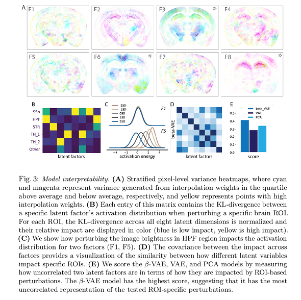
Note 1: essentially, the color code in subfigure A provides a measure of which pixels are strongly modified when a specific latent factor changes. Note 2: stars mark factors that seem to encode outliers more prominently.
Conclusions
The work presents:
- A \(\beta\)-VAE that can model high-resolution structural brain images
- A bi-directional approach for revealing relationships between brain regions and latent factors in the proposed VAE framework.
- A demonstration that structured perturbations to both image inputs and the latent space can reveal biologically meaningful variability.
Comments
Authors acknowledge that more complex VAE variants could further facilitate latent factor distentanglement and interpretability.