Introduction

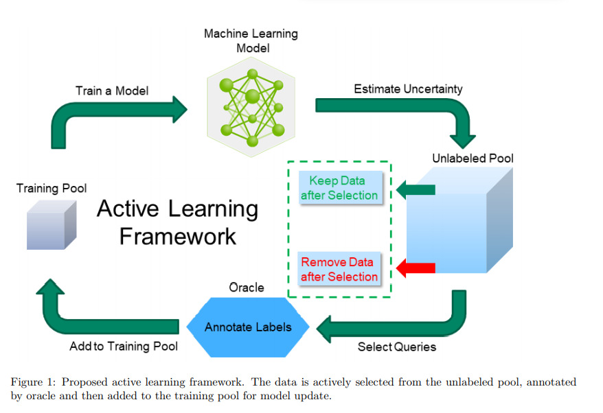
Authors explore active learning for the task of segmentation of medical imaging data sets.

They propose the following 3 contributions:

1. A query by committee method based on an adaptation of Stein variational gradient descent (SVGD) for Dice log-likelihood loss.
2. Increasing frequency of uncertain samples in the training set by allowing the model to sample image multiple times.
3. Uncertainty estimation using mutual information between labeled set and unlabeled set to increase diversity in the training set (This regulates contribution 2.)

Methods

Querying

Authors use a query by committee framework which uses multiple models to estimate uncertainty. This requires a committee of models which is implemented with a Stein variational gradient descent (SVGD). SVGD is a joint optimization technique for ensemble models. M copies of model parameters, \(\Theta = \{\theta^q\}^M_{q=1}\), referred to as particles are jointly optimized.

Each particle is updated by \(\theta_{k+1} \leftarrow \theta_k + \epsilon_k \phi(\theta_k)\) where \(\phi(\theta_k)\) is

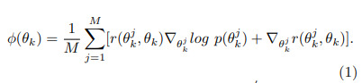
\(r(\theta, \theta')\) is a positive definite radial basis function (RBF). Each particle is trained to reach a unique local minima by repulsive forces between each particle (last term in (1)).

Authors adapt SVGD to Dice log-likelihood loss which is defined as \(log(\mathcal{L}_{dice})\) (standard fomulation of SVGD uses entropy loss).

Uncertainty estimation

Authors use an entropy based epistemic (model) uncertainty for every 3D voxel defined by

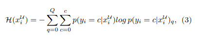
this is computed for every particle \(q\) and every sample \(x_i\) in the unlabeled set.

Authors also add a second term to the score of a sample based on mutual information with samples from the labeled set.

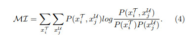
where \(P(x^{\mathcal{T}}_i, x^{\mathcal{U}}_j)\) is the joint probability and \(P(x^{\mathcal{T}}_i)\), \(P(x^{\mathcal{U}}_j)\) are marginal probabilities with respect to the histograms of the two images for training samples \(x^{\mathcal{T}}_i\) and un-labeled samples \(x^{\mathcal{U}}_j\)

The epistemic uncertainty and mutual information are normalized and the final score is calculated according to:

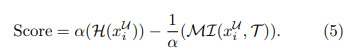
The mutual information term is subtracted because a lower score for mutual information indicates more diversity.

Deleting samples

Contrary to other active learning methods, the authors propose leaving samples in the Unlabeled pool once they are labeled. Therefore, if the model is still uncertain about this sample in subsequent steps, it can be sampled once again but will not require more labeling.

Data

Authors test their method on 2 datasets:

• Pancreas and tumor segmentation based on 3D computed tomography (CT) volume
  • Samples processed by cubic 48x48x48 patches
  • Down-sampled to 4.0 mm isotropic resolution
  • Data clipped in the range -87 to 199 (Hounsfield units) and normalized to [0, 1].
• Hippocampus segmentation of two different regions of interest based on T1-weighted magnetic resonance imaging (MRI)
  • Samples processed by 64x64x64 volumes
  • Normalized with clip range used was 0 to 2048.

Results

The following table shows the hyper-parameters used for the active learning experiments.

Hyper-parameters	Hippocampus	Pancreas
Learning rate	0.001	0.0004
Batch size (volumes)	8	8
Active iterations	40	40
Number of models (SGVD)	5	5
Training steps per active step	1500	10000
Set size (subjects) (init train/U/val/test)	10/153/50/50	20/201/30/30
Queries per active step	1	5

Authors compare different combinations of their methods with standard ensemble methods. All experiments were performed with 5 different random seeds.

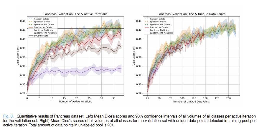
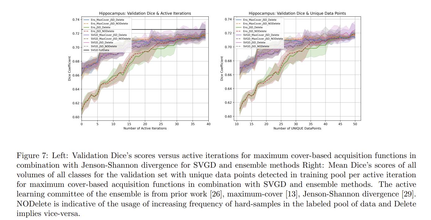
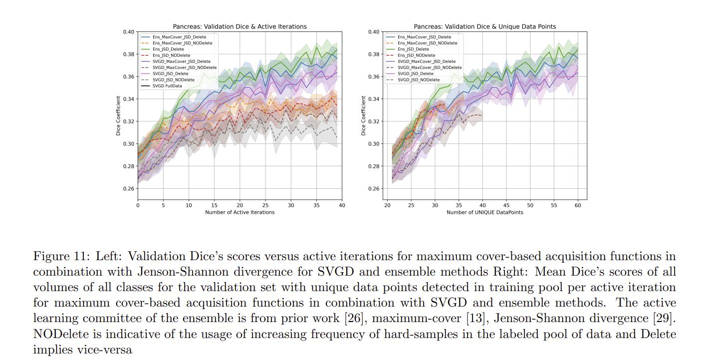
Authors also compare their method to maximum cover¹ and Jenson-Shannon divergence² acquisitions functions.

Conclusions

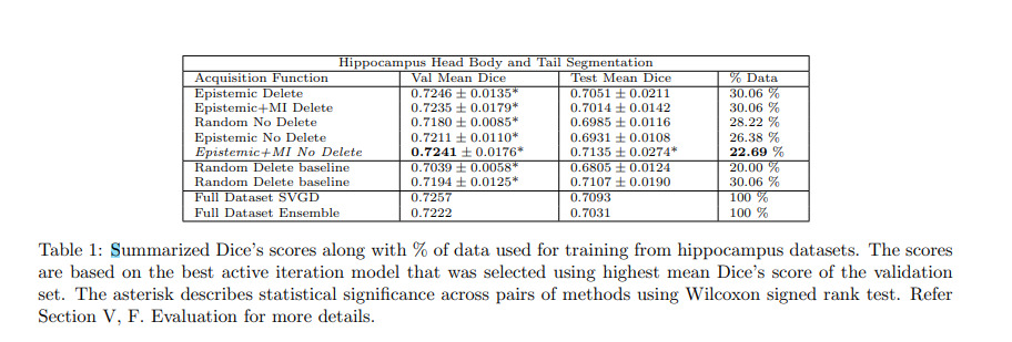
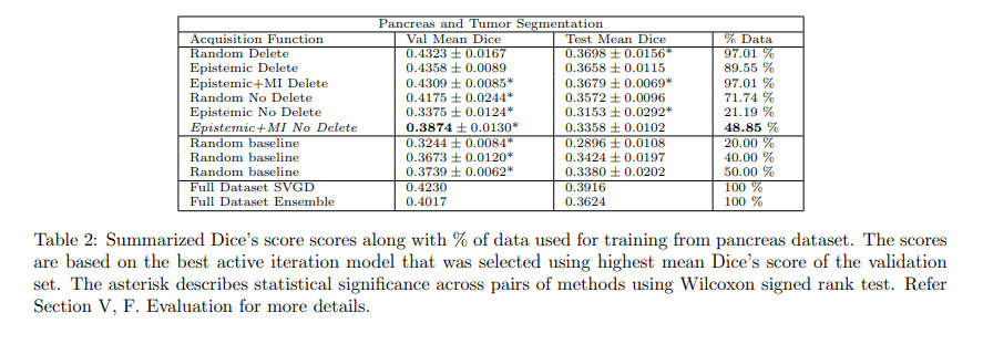
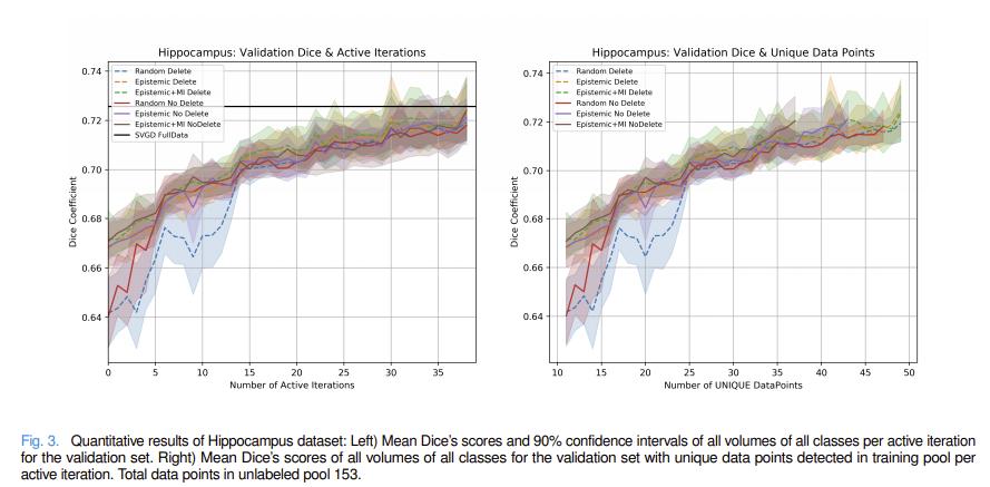
Authors conclude that their methods work well for the hippocampus dataset but not for the pancreas dataset. Authors argue that this shows that active learning methods are very dataset dependent and that the discrepancy between the results of the two datasets could be explained by the fact that hippocampus samples were processed by the entire volume while the pancreas samples were split into patches.

Comments

The authors mention that they used a lighter version of UNet for rapid experiment for faster testing and do not use any data augmentation to only evaluate the active learning methods.

Training time was 160 and 60 GPU hours for pancreas and hippocampus datasets respectively.

References