Highlights

A similarity measure is introduced to measure the difference between representations created by trained neural networks.
They compare to other similarity measures and show theirs is better at measuring similarity.
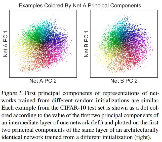
They stress out that an effective similarity method could answer important questions such as (1) Do deep neural networks with the same architecture trained from different random initializations learn similar representations? (2) Can we establish correspondences between layers of different network architectures? and (3) How similar are the representations learned using the same network architecture from different datasets?
Here is a video presentation of the paper by one of the authors.

Introduction

Let \(X \in \mathbb{R}^{n \times p_1}\) denote a matrix of activations of \(p_1\) neurons for \(n\) samples, and \(Y \in \mathbb{R}^{n \times p_2}\) denote a matrix of activations of \(p_2\) neurons for the same \(n\) samples (assume \(p_1 \leq p_2\).). The authors look for a scalar similarity index \(s(X,Y)\) that can be used to compare representations within and across neural networks, in order to help visualize and understand the effect of different factos of variation in deep learning.

Invariance of the similarity measure

To invertible linear maps

A similarity index is invariant to invertible linear maps if \(s(X,Y) = s(XA,YB)\) for any full rank \(A\) and \(B\). The authors prove that a similarity index with this invariance gives the same result for any representation of width greater than or equal to the dataset size, i.e., when \(p_2 > n\).

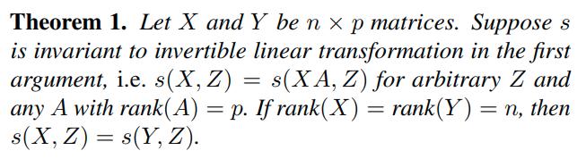
They also remark that invariance to invertible linear maps implies that the scale of directions in activation space is irrelevant and that such invariance will result in a similarity that assigns the same score to networks that match only in large principal components or networks that match only in small principal components.

To orthogonal transformations

This invariance is defined as \(s(X,Y)=s(XU,YV)\) for full-rank orthonormal matrices \(U\) and \(V\) such that \(U^T U = I\) and \(V^T V = I\).

Similarity indexes invariant to orthogonal transformations remain well-defined when \(p_2 > n\).
Invariance to orthogonal transformations implies invariance under permutations, which is more suited to accommodate neural network representations.

The authors also note that, in the linear case, orthogonal transformations of the input do not affect the dynamics of gradient descent training, and for neural networks initialized with rotationally symmetric weight distributions (i.i.d. Gaussian weight initialization), training with fixed orthogonal transformations of activations yields the same distribution of training trajectories as untransformed activations. The latter is not true for arbitrary linear maps instead of orthogonal transformations.

To isotropic scaling

Isotropic scaling invariance is by definition \(s(X,Y)=s(\alpha X, \beta Y)\) for any \(\alpha, \beta \in \mathbb{R}^+\).

They note that a similarity index that is invariant to both orthogonal transformations and non-isotropic scaling (rescaling of individual features) is invariant under invertible linear transformations.

Comparing similarity structures

Dot product-based similarity

The dot product between examples is related to the dot products between features by the formula

\[<vec(XX^T),vec(YY^T)> = tr(XX^TYY^T) = \| Y^TX \|_F^2.\]

The elements of \(XX^T\) and \(YY^T\) are dot products between the representations of the \(i^{\text{th}}\) and \(j^{\text{th}}\) examples and indicate the similarity between these examples according to the respective networks.
The left-hand side of this equation measures the similarity between the inter-example similarity structure.
The right-hand side measures the similarity between features from \(X\) and \(Y\).

Hilbert-Schmidt independence criterion

Define \(H=I_n- \dfrac{1}{n} \textbf{1} \textbf{1}^T\). The empîrical estimator of Hilbert-Schmidt Independence Criterion (HSIC) with kernels \(k\) and \(\ell\) defining matrices \(K_{i,j} = k(x_i,x_j)\) and \(L_{i,j} = \ell(x_i,x_j)\) is by definition:

\[HSIC(K,L) = \dfrac{1}{(n-1)^2} tr(KHLH).\]

For the kernels \(k(x,y)=\ell(x,y)=x^Ty\), one obtains \(HSIC(K,L) = \| cov(X^T,Y^T) \|_F^2\).
When \(k\) and \(\ell\) are universal kernels, \(HSIC(K,L)=0\) implies independence.
HSIC is not an estimator of mutual information.
HSIC is equivalent to maximum mean discrepancy between the joint distribution and the product of the marginal distributions.
HSIC with a specific kernel family is equivalent to distance covariance.

Centered kernel alignment

HSIC is not invariant to isotropic scaling. This can be fixed by normalizing:

\[CKA(K,L) = \dfrac{HSIC(K,L)}{\sqrt{HSIC(K,K) HSIC(L,L)}}.\]

For linear kernels, CKA is equivalent to the RV coefficient and to Tucker’s congruence coefficient.

Kernel selection

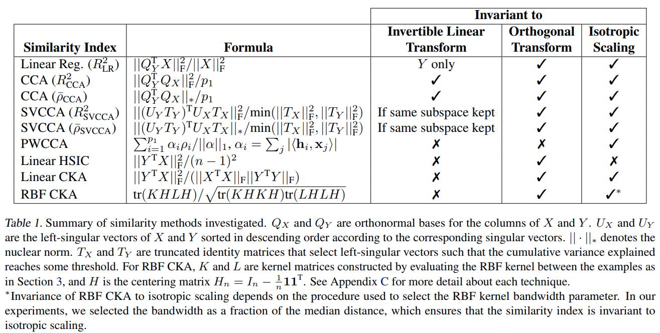
The authors propose as a similarity measure the CKA with hte RBF kernel \(k(x_i,x_j) = exp(-\| x_i-x_j \|_2^2 /(2 \sigma^2))\). The bandwidth \(\sigma\) controls the extent to which similarity of small distancesis emphasized over large distances.

The authors chose \(\sigma\) as a fraction of the median distance between examples.

For given representations \(X\) and \(Y\) we let \(Q_X = X(X^TX)^{-1/2}\) and \(Q_Y = Y(Y^TY)^{-1/2}\).

Linear Regression. One can fit every feature in \(Y\) as a linear combination of features from \(X\). The total fraction of variance is given by the fit: \(R^2_{LR} = \dfrac{\| Q_Y^T X \|_F^2}{\| X \|_F^2}.\)
Canonical Correlation Analysis (CCA). Canonical correlation changes the bases in which \(X\) and \(Y\) are expressed to maximize the correlation. For \(1 \leq i \leq p_1\), the \(i^{\text{th}}\) canonical correlation coefficient is defined as: \(\rho_i = max_{w_X^i,w_Y^i} corr(Xw_X^i, Yw_Y^i)\) where we restrict to the perpendicularity conditions: \(Xw_X^i \perp X w_X^j\) and \(Yw_Y^i \perp Yw_Y^j\) for all \(j>i\). The canonical variables are \(Xw_X^i\) and \(Yw_Y^i\).

The authors consider the following statistics of the goodness of fit of CCA: \(R_{CCA}^2 = \dfrac{\| Q_Y^T Q_X \|^2_F}{p_1}, \text{ and }\) \(\rho_{CCA} = \dfrac{\| Q_Y^T Q_X \|_*}{p_1}.\) Here \(\| - \|_*\) denotes the nuclear norm which is the sum of the singular values.

SVCCA. One extra thing that can be built on top of CCA is to perform CCA on the truncated singular value decompositions of the representations \(X\) and \(Y\). It has been demonstrated that SVCCA keeps enough principal components of the input matrices to explain a fixed proportion of the variance, and drops the remaining components.
Projection-Weighted CCA. Let \(x_j\) be the \(j\)-th column of \(X\) and \(h_i=X w_X^i\), and also \(\alpha_i = \sum_j \mid <h_i,x_j> \mid\). Projection-weighted canonical correlation (PWCCA) is given by

\[\rho_{PW} = \dfrac{\sum_i^c \alpha_i \rho_i}{ \sum_i \alpha_i}.\]

The authors derive a relation of PWCCA to linear regression (Appendix C.3).

Neuron Alignment Procedures. The authors mention other works where alignment between individual neurons is analyzed. Other works have found that the maximum matching subsets are very small for intermediate layers.
Mutual Information. This measure is invariant under any invertible map, not only linear. The authors argue that this is not a good measurement for similarity between representations.

Linear CKA versus CCA and Regression

The authors expose relations between CKA, CCA and linear regression, the first of which is \(R^2_{CCA} = CKA(Q_X Q_X^T, Q_YQ_Y^T) \sqrt{p_2/p_1},\) the second one: \(R^2_{LR} = CKA(XX^T, Q_Y Q_Y^T) \dfrac{\sqrt{p_1} \| X^TX \|_F}{\| X \|_F^2}.\) A further simplification of these can be computed if we consider the SVD (singular value decomposition) of \(X=U_X \Sigma_X V_X^T\) and \(Y=U_Y \Sigma_Y V_Y^T\). If \(u_X^i\) denotes the \(i\)-th eigenvector of \(XX^T\) (i.e., the \(i\)-th column of \(U_X\)), then \(R_{CCA}^2 = \sum_{i=1}^{p_1} \sum_{j=1}^{p_2} <u_X^i,u_Y^j>^2 /p_1.\) If \(\lambda_X^i\) denotes the \(i\)-th eigenvalue of \(XX^T\), then \(CKA(XX^T,YY^T) = \dfrac{ \sum_{i=1}^{p_1} \sum_{j=1}^{p_2} \lambda_X^i \lambda_Y^j <u_X^i,u_Y^j>^2}{ \sqrt{\sum_{i=1}^{p_1} (\lambda_X^i)^2} \sqrt{\sum_{j=1}^{p_2} (\lambda_Y^j})^2 }.\)

One noticeable advantage of CKA is that it does not require the computation of the SVD.

Results

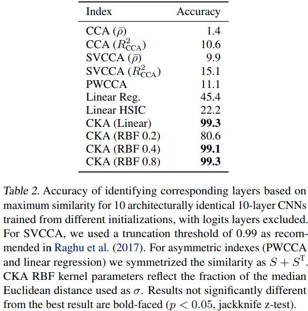
Sanity check

The authors propose a sanity check for similarity indexes:

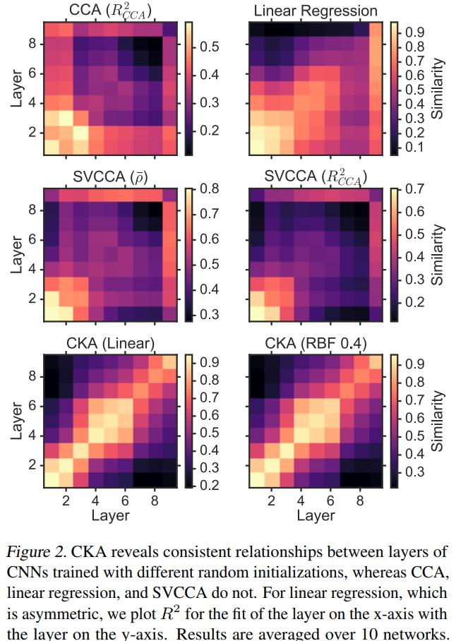
Given a pair of architecturally identical networks trained from different random initializations, for each layer in the first network, the most similar layer in the second network should be the architecturally corresponding layer.

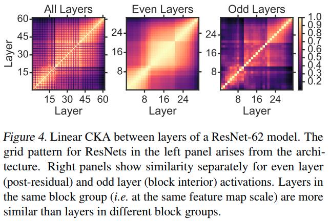
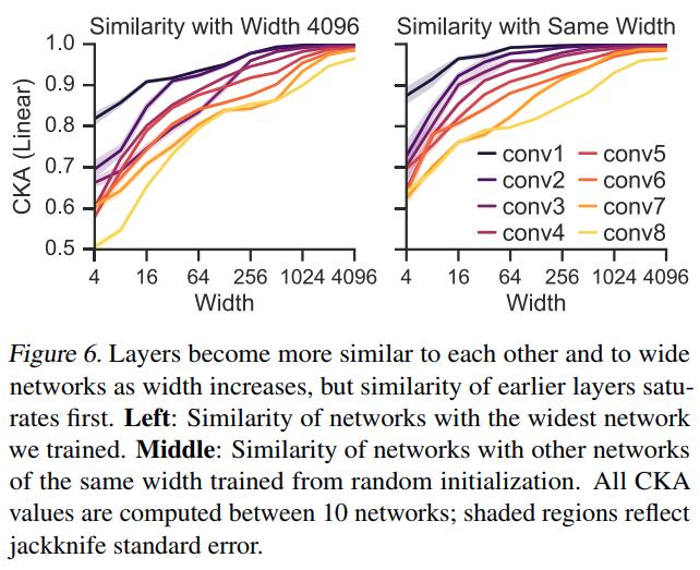
Using CKA to understand network architecture

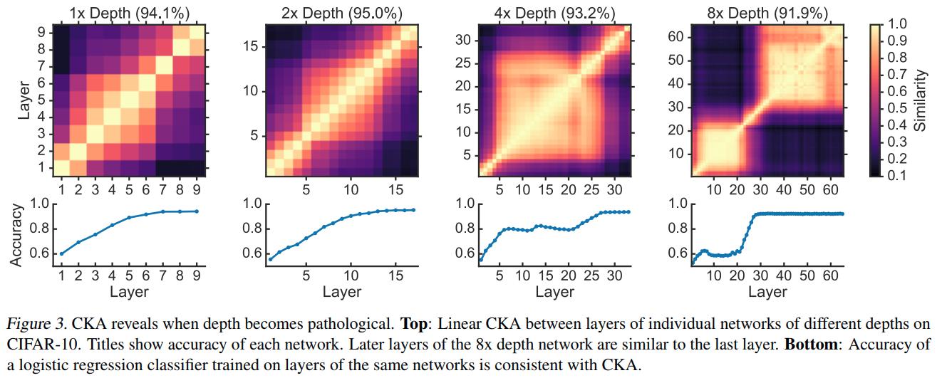
The authors validate that the later layers do not refine the representation by training an \(\ell^2\)-regularized logistic regression classifier on each layer of the network.

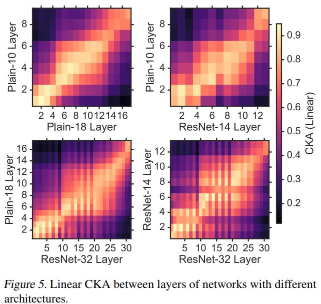
CKA indicates that, as networks are made deeper, the new layers are effectively inserted in between the old layers. The authors show that other similarity indexes fail to reveal meaningful relationships between different architectures in Appendix F.5.

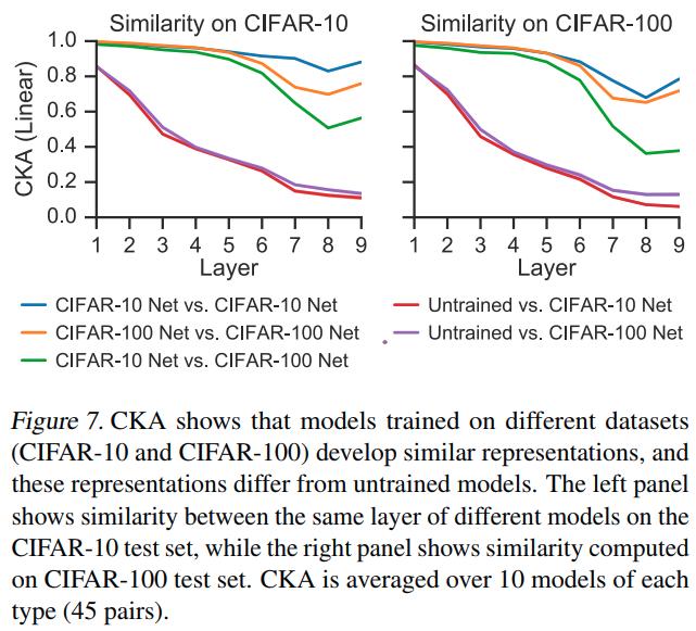
Similar representations across datasets

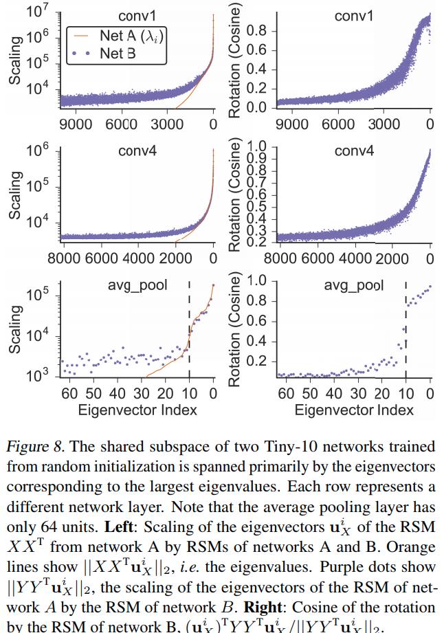
Analysis of the shared subspace

Conclusions

Measuring similarity between the representations learned by neural networks is an ill-defined problem, since it is not entirely clear what aspects of the representation a similarity index should focus on.
CKA consistently identifies correspondences between layers, not only in the same network trained from different initializations but across entirely different architectures.
CKA reveals an intuitive notion of similarity, that is, neural networks trained from different initializations should be similar to each other.
Kernel selection is still a mystery.