Highlights

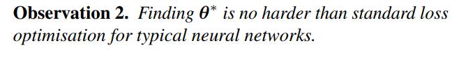
They prove two theorems stating that, independently of the data sets:

1.- Every finite-dimensional pattern can be found as the loss landscape of a sufficiently deep and wide neural network. This property transfers to the test data.
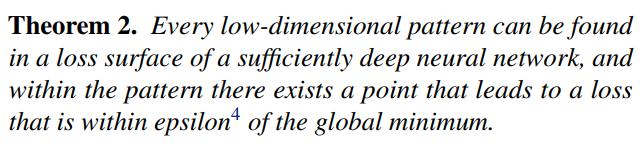
2.- This can be done such that the minimum of the found pattern is arbitrarily close to a global minimum of the network.

Introduction

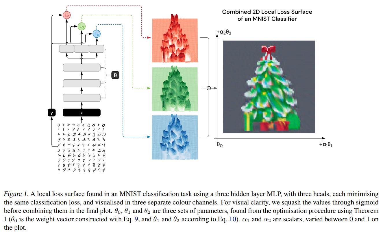
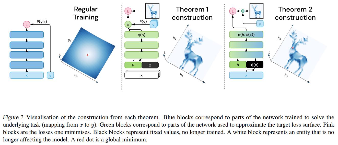
Let \(\mathcal{T}\) be a \(z\)-dimensional function. The goal is to find parameters \(\theta_0\) and \(z\) directions \(\theta_i\) in the parameters space such that the training loss in each point of the set \(\{ \theta_0 + \sum_i \alpha_i \theta_i : \alpha_i \in [0,1] \}\) is approximately equal to \(\mathcal{T}\).

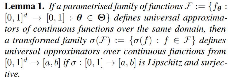
Losses as universal approximators

Ideas of the proof:

Let \(\epsilon >0\).
Set all weights of the first hidden layer equal to zero.
The non-zero weights still form a universal function approximator (using the biases as the inputs).
Use Lemma 1 to get parameters \(\theta_\epsilon (\mathcal{T})\) to replace the non-zero weights approximating \(\mathcal{T}\).
Use \(\sigma(p) := \frac{1}{N} \sum_i \ell(p,\mathbf{y}_i)\) for the Lemma.
The loss surface pattern is \(\theta_\epsilon^*(h_1,...,h_z) := \{ \mathbf{0}, [h_1,...,h_z,0,...,0], \theta_\epsilon (\mathcal{T}) \}\)

Other things to notice:

The initial position is \(\theta_0 = \{ \mathbf{0}, [0,...,0], \theta_\epsilon (\mathcal{T}) \}\).
The directions are \(\theta_i = \{ \mathbf{0}, [0,...,0,1,0,...,0], \mathbf{0} \}\).
This is why \(L(\theta_0 + \sum_i \alpha_i \theta_i)\) approximates \(\mathcal{T}(\alpha_1,...,\alpha_z)\).
The pattern is axis aligned.

Since the prediction depends on the dataset only through the marginal distribution of the output labels.
This implies that the loss surface patterns will transfer to other datasets, as long as the loss function is the same and the marginal distribution coincides (so datasets with the same number of classes like MNIST and CIFAR-10).

This is a consequence of the proof of Theorem 1.
Only need to train the network obtained after removing the first layer.

Ideas of the proof:

Set to zero all weights in the first layer pointing to the first \(z\) neurons of the first hidden layer.
This is again a universal approximator.
The approximate minimum will be at \(\mathbf{h}^* := argmin_{\mathbf{h} \in [0,1]^z} \mathcal{T}(\mathbf{h})\).
It has to be noticed, that in this case, the result will not transfer to the test data.

Conclusions

The loss surfaces of neural networks contain every low-dimensional pattern.
This holds for any dataset.
This transfers from training data to test data.
This can be found as easily as supervised learning.
The patterns can be guaranteed to be axis aligned.
The patterns can be modified to have loss value close to a global minimum.

And one very important thing to keep in mind.

Be cautious if you consider adding regularisation in the form of local loss surface geometry preferences on low-dimensional sections since networks might be able to \(\textbf{cheat}\) and satisfy these constraints independently from their operation over input space.