G-SGD: Optimizing ReLU neural networks in its positively scale-invariant space
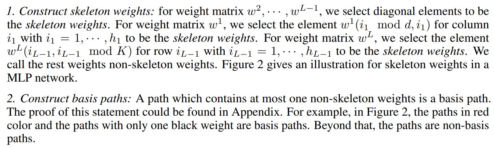
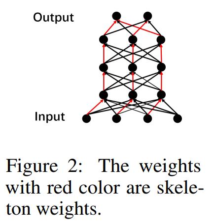
Highlights
- ReLU neural networks are optimized in a space that is invariant under positive rescaling. This space is also sufficient to represent ReLU networks.
- This is achieved by exploiting dependencies between the values of all the paths from the input layer to the output layer.
- This method only works for MLPs and CNNs with the same number of neurons per hidden layer.
Introduction
Let \(N_w(x): \mathcal{X} \to \mathcal{Y}\) denote a L-layer multi-layer perceptron with weights \(w \in \mathcal{W} \subset \mathbb{R}^m\), input space \(\mathcal{X} \subset \mathcal{R}^d\) and output space \(\mathcal{Y} \subset \mathcal{R}^K\). In the \(l\)-th layer, there are \(h_l\) neurons. We denote the \(i_l\)-th node by \(O_{i_l}^l\) and its value on a forward pass by \(o_{i_l}^l\). The weight matrix between layers \(l-1\) and \(l\) is denoted \(w^l\), and the weight connecting neurons \(O_{i_l-1}^{l-1}\) and \(O_{i_l}^l\) is denoted \(w^l(i_{l-1},i_{l})\). The path from the input node \(O_{i_0}^0\) to the output node \(O_{i_L}^L\) passing through the nodes \(O_{i_0}^0,...,O_{i_L}^L\) is denoted by \((i_0,...,i_L)\). The network structure can be regarded as a directed graph \((\mathcal{O},E)\), with vertices \(\mathcal{O}=\{ O_1,...,O_{H+d+K} \}\) and edges \(E\), where H is the number of hidden neurons and \(|E|=m\).
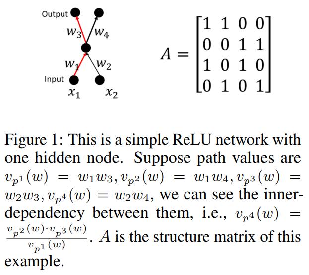
A path is represented by a vector \(p=(p_1,...,p_m)^T\) and if edge \(e\) is contained in path \(p\), then \(p_e=1\) and otherwise \(p_e=0\). These vectors have \(L\) entries that are non-zero. The value of path \(p\) is defined as \(v_p(w)= \prod_{i=1}^m w_i^{p_i}\). The set of all such paths is denoted \(\mathcal{P}\). Finally, the activation status of path \(p\) is \(a_p(x;w)=\prod_{j:p_{e_{ij}}=1} \mathbb{I}\big( o_j(x;w) > 0 \big)\).
Positively Scale-Invariant Space
-
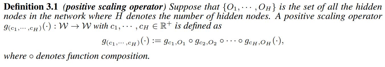
The group acting on weight space via positive scale invariance is the group \(\mathcal{G}=\{ g_{(c_1,...,c_H)}(\cdot) : c_1,...,c_H \in \mathcal{R}^+ \}\).
-
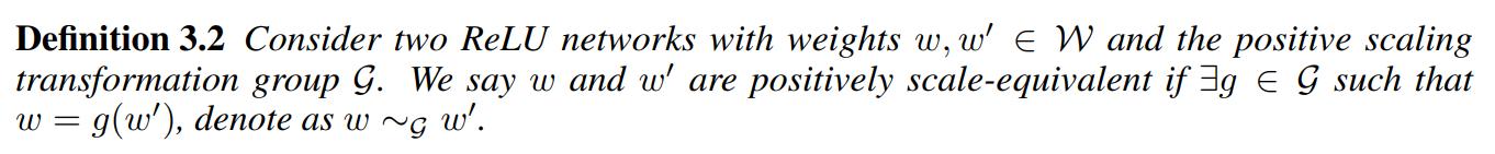
If \(w=g(w')\) for some \(g\in \mathcal{G}\) then \(N_w(x)=N_{w'}(x)\) for all input vector \(x\).

-
Based on this, the authors propose to optimize the values of paths instead of weights.
-
They consider the set of path vectors \(\mathcal{P} \subset \{ 0,1 \}^m\).
-
The matrix composed by all paths is denoted A and its called the structure matrix of the ReLU network. It is of size \(m \times n\).
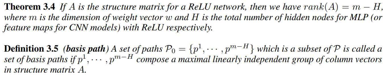
- Given the structure matrix and the values of basis paths, the values of the weights cannot be determined unless the values of free variables are fixed.


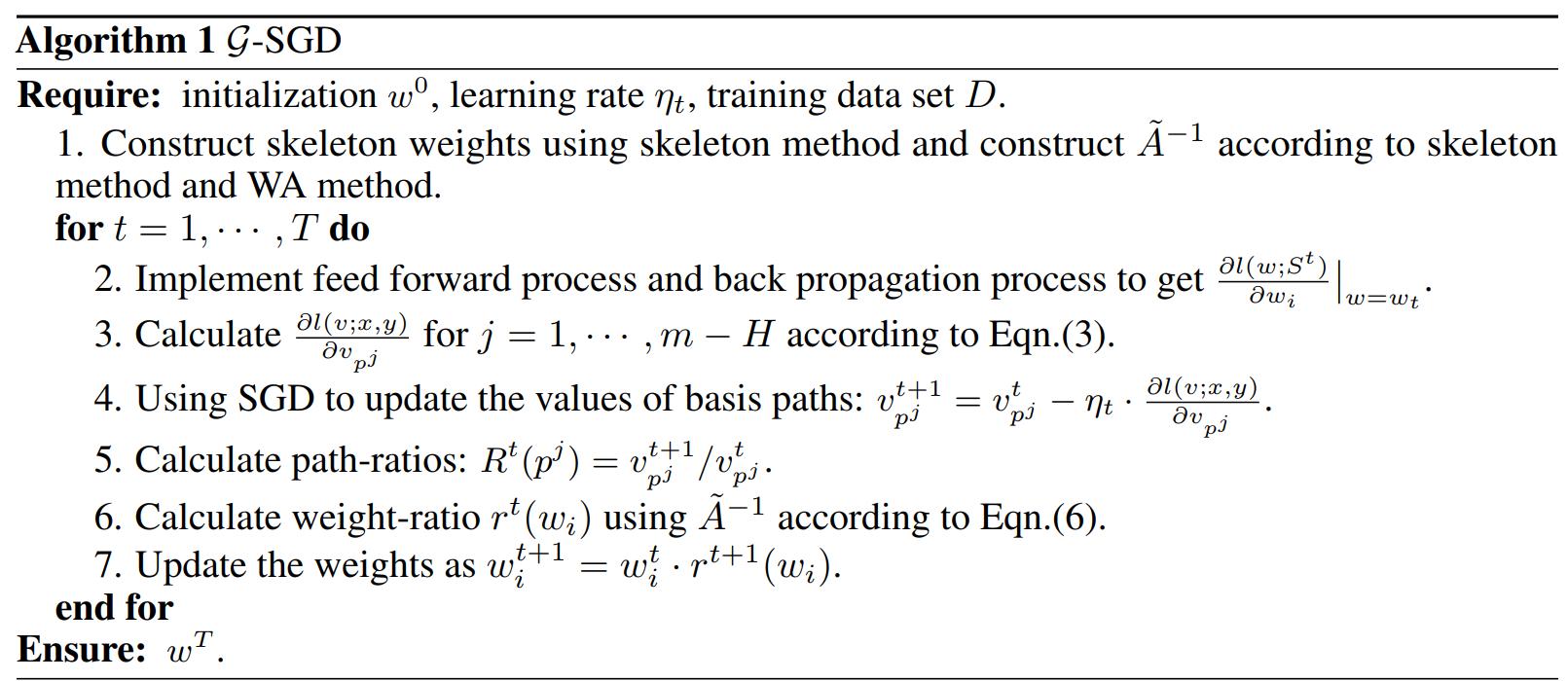
\(\mathcal{G}\)-SGD optimization algorithm
Three methods are required to obtain the \(\mathcal{G}-SGD\) algorithm.
Skeleton Method
For an MLP of depth L and width h, this method constructs the skeleton weights.
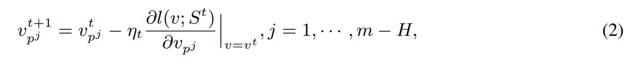
The update rule for basis paths is:
Inverse Chain-Rule (ICR) Method
The end goal of this method is to compute the gradient with respect to the basis paths in terms of the gradient with respect to the weights. By the chain rule we have the following equation:
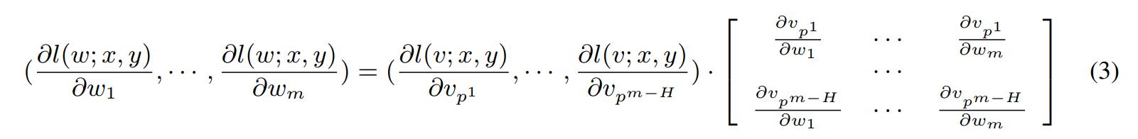
Observe that
- \(\dfrac{\partial v_p}{\partial w_e} = \dfrac{v_p}{w_e}\) if the edge \(e\) is contained in the path \(p\), and \(\dfrac{\partial v_p}{\partial w_e} = 0\) if not.
- Each non-skeleton weight is contained in only one basis path. This means that there is only one non-zero element in each column of the matrix in (3).
Weight-Allocation (WA) Method
With the previous two methods, the update rule for basis paths is computed. But a way to update the weights is required, and this is the purpose of weight-allocation. For this we need the following definitions:
- The path-ratio at iteration t: \(R^t(p^j):= v_{p_j}^t/ v_{p_j}^{t-1}\).
- The weight-ratio at iteration t: \(r^t(w_i)=w_i^t/w_i^{t-1}\).
- \(w \odot p^j := \prod_{i=1}^m w_i^{p_i^j}\).
Observe that \(v_{p^j}(w) = w \odot p^j\) and that \(R^t(p^j) = r^t(w) \odot p^j\). The operation \(\odot\) can be extended to matrices too in the obvious way.

where \(A'=(p^1,...,p^{m-H})\). Assume that \(w_1,...,w_H\) are the skeleton weights. The vector \(( R^t(p^1)),..., R^t(p^{m-H}))\) is completed to an m-dimensional vector by adding 1’s at the beginning. Define \(\widetilde{A}:= [B,A']\) with \(B=[I,0]^T\), where I is an \(H \times H\) identity matrix and \(0\) is an \(H \times m\) zero matrix. Then
- \[rank( \widetilde{A} ) = m\]


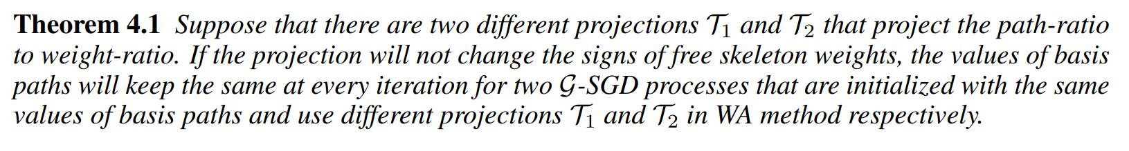
- This is not the only way to obtain weight-ratios from path-ratios. But the authors prove the following:
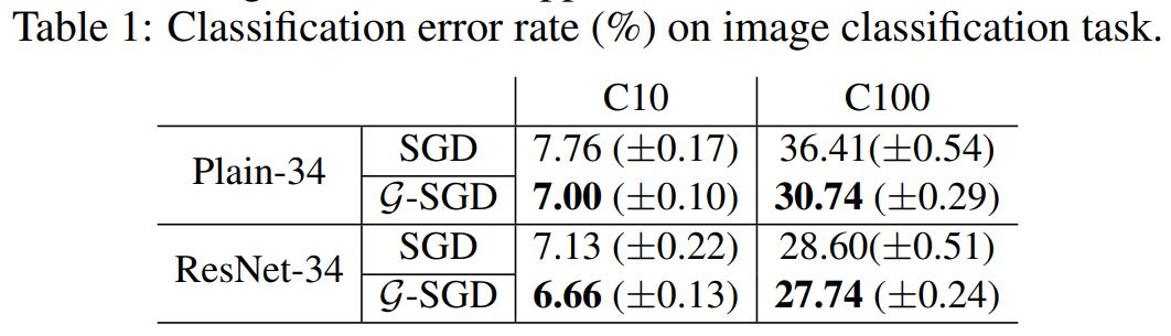
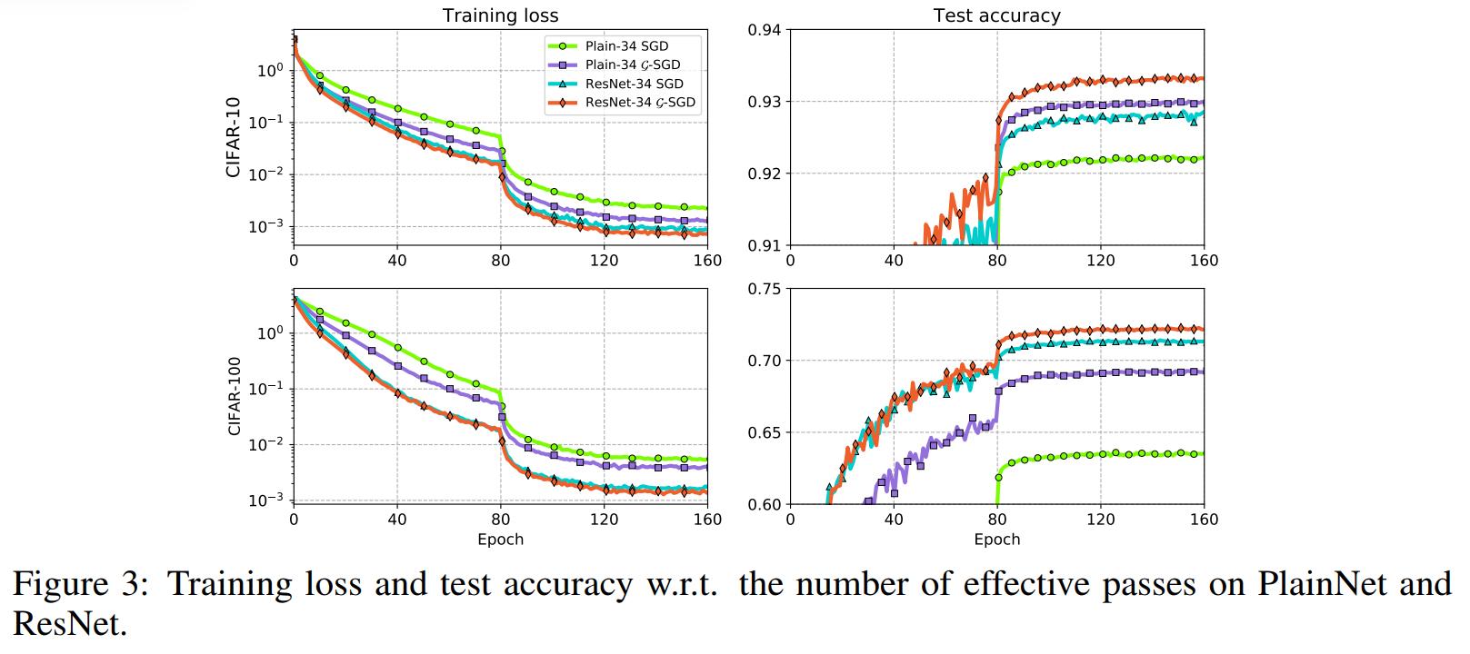
Experiments
Each curve is the average of 5 training curves.
- For CNNs the following results are reported:
-
The authors claim that due to the skip connections there are no basis paths for the whole ResNet model. They also claim that there is no positive scale invariance across residual connections because it breaks the structure that they construct.
-
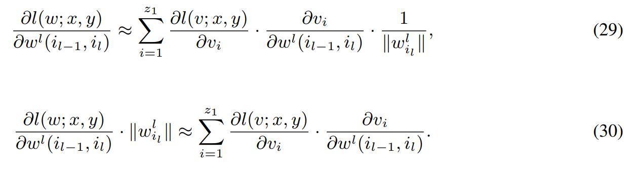
They also treat batch-norm separately. The following approximation is considered:
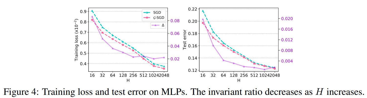
- For MLP with two hidden layers of size H, where \(\bigtriangleup\) denotes the performance gap between \(\mathcal{G}-SGD\) and vanilla SGD. These curves are produced over the data set Fashion-MNIST
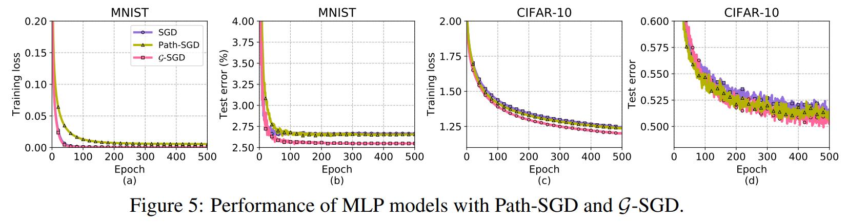
- Finally, they compare with Path-SGD:
Conclusions
-
The use of the dependencies between paths in a ReLU network can be exploited to produce better optimization when compared with usual SGD.
-
It is not clear how they obtain the skeleton weights for CNNs.
-
They do not compare with other optimization algorithms like momentum or Adam, only with vanilla SGD and path-SGD.