Disentangled Representation Learning in Cardiac Image Analysis
Highlights
- New network architecture (SDNet) that factorizes 2D medical images into spatial anatomical factors and non-spatial modality factors;
- Various experiments to show that the learned representation is well-suited to a variety of image analysis tasks,
including:
- semi-supervised segmentation
- multi-task segmentation and regression (e.g. Left Ventricular Volume estimation)
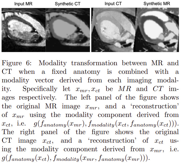
- image-to-image synthesis
Introduction
Learning a decomposition of data into a spatial content factor and a non-spatial style factor has been a focus of recent research in computer vision[…].
This focus can be explained by the advantages of such a representation:
-
Meaningful representation of the anatomy that can be generalized to any modality
-
Suitable format for pooling information from various imaging modalities
Methods
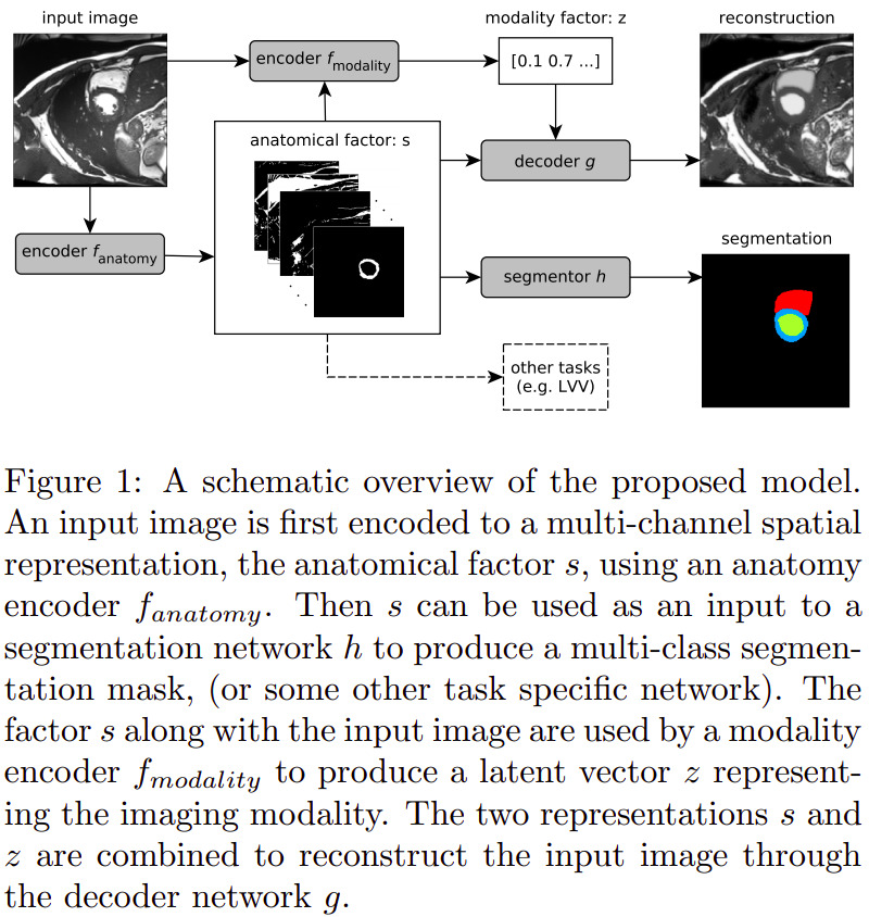
Spatial Decomposition Network (SDNet)
The SDNet can be seen as an autoencoder that learns multiple factors, namely:
- \(s = f_A (x)\): a multi-channel output of binary maps, representing the anatomical components
- \(z = f_M (x)\): the \(Q(z \vert X)\) multivariate Gaussian as in a standard VAE, representing the modality components
Other sub-networks are added to provide feedback over multiple tasks, with varying degrees of supervision:
- \(g\): a self-supervised decoder that tries to reconstruct the input image from its \(s\) and \(a\) decomposition;
- \(h\): a segmentor network that predicts the cardiac segmentation from \(s\).
- When a ground truth is available for the current image, \(h\) is trained using a standard Dice loss;
- Otherwise, the training is semi-supervised through a GAN-like adversarial loss, where a discriminator network tries to predict whether a segmentation mask was predicted by \(h\) or comes from a pool of groundtruth segmentations.
The overall loss function is the following weighted sum (determined empirically):
\[L = \lambda_1 L_{KL} + \lambda_2 L_{segm} + \lambda_3 L_{adv} + \lambda_4 L_{rec} + \lambda_5 L_{z_{rec}}\]where \(L_{KL}\) and \(L_{rec}\) make up the autoencoder’s self-supervision, and \(L_{segm}\) and \(L_{rec}\) correspond to the aforementioned segmentation supervision or semi-supervision. The additional factor is \(L_{z_{rec}}\), which is enforces a modality factor reconstruction:
\[L_{z_{rec}} = \mathbb{E}_{z,y} [\|z - f_{modality}(y, f_{anatomy}(y))\| _{1}]\]where \(y\) is an image produced using a random \(z\) sample. This is done to avoid a posterior collapse, where the decoder would ignore parts or the totality of the modality factor.
Data
Semi-supervised segmentation
- Training subset of the ACDC dataset:
- 1920 images with manual segmentations (ED and ES) and 23,530 images with no segmentations
- Edinburgh Imaging Facility QMRI: 26 healthy volunteers with around 30 cardiac phases each, acquired on a 3T scanner
- 241 images with manual segmentations (ED) and 8353 images with no segmentations
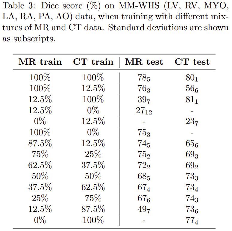
Multimodal segmentation and modality transformation
- Data from the 2017 Multi-Modal Whole Heart Segmentation (MM-WHS) Challenge: 20 cardiac CT/CT angiography (CTA) volumes
and 20 cardiac MRI volumes
- 3626 MR and 2580 CT images, all with manual segmentations of seven heart structures: myocardium, left atrium, left ventricle, right atrium, right ventricle, ascending aorta and pulmonary artery
Modality estimation
-
cine-MR and CP-BOLD images of 10 canines[…]. Two almost identical sequences with the only difference that CP-BOLD modulates pixel intensity with the level of oxygenation present in the tissue.
- 129 cine-MR and 264 CP-BOLD images with manual segmentations from all cardiac phases
Results
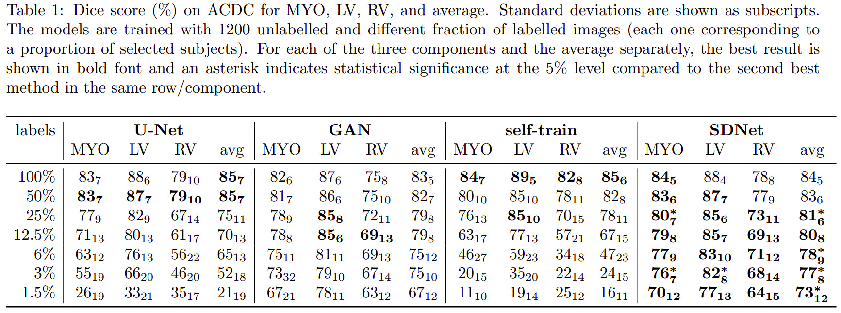
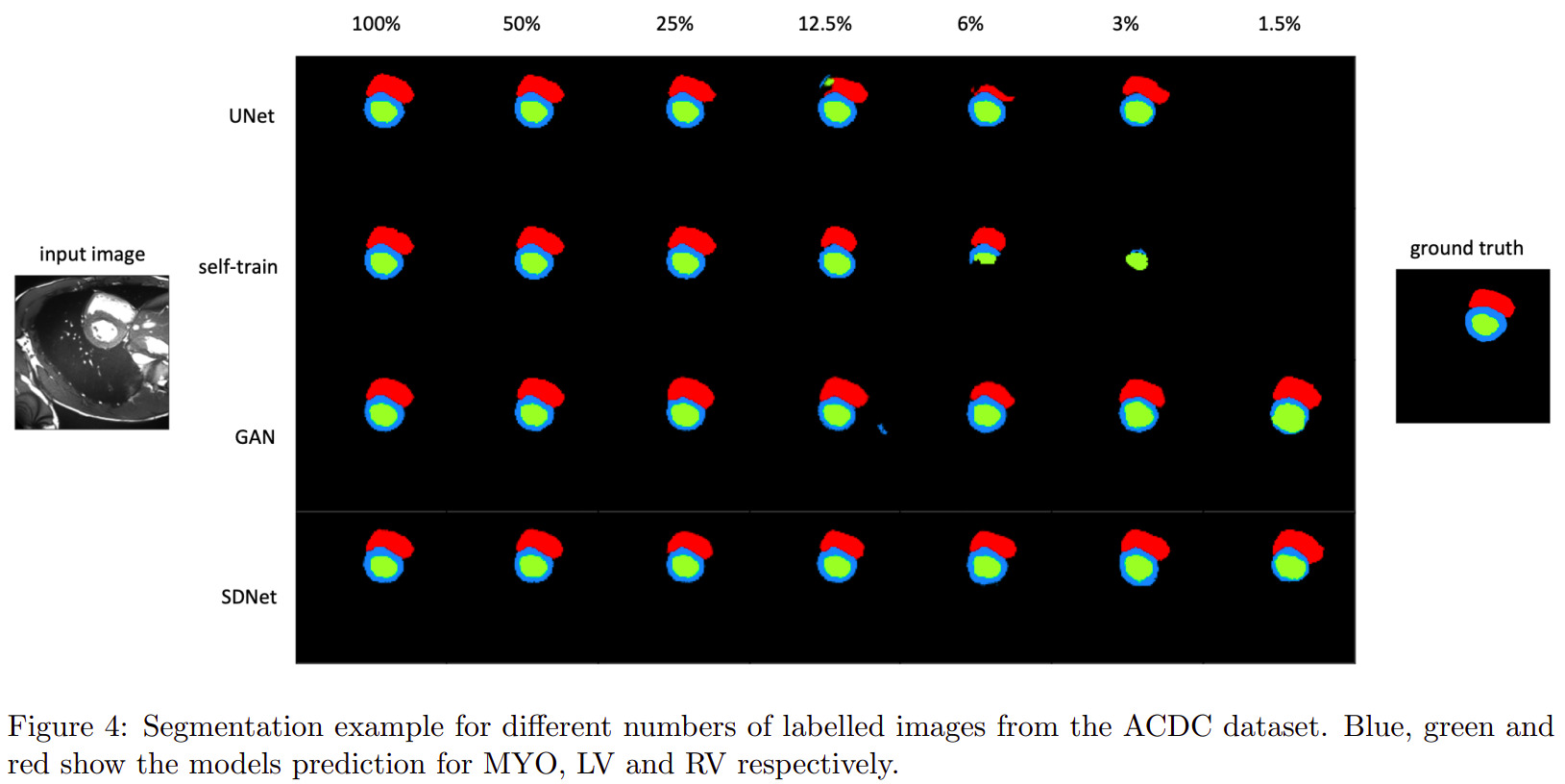
Semi-supervised segmentation
Multimodal learning
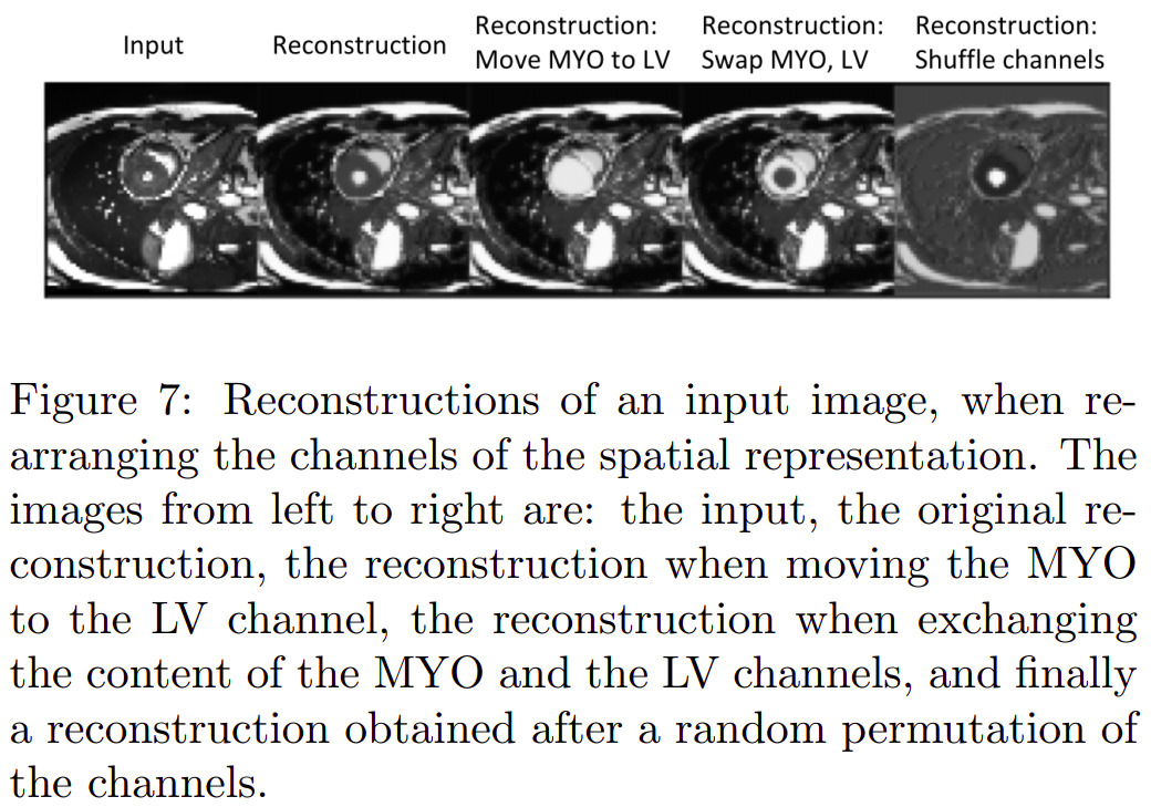
Latent space arithmetic
Others
Other experiments were also conducted relative to modality type estimation (from modality factors) and modality factor traversal (named factor sizes in the paper).
Remarks
- The authors present a lot of details about their design choices, so it seems possible to reproduce accurately their experiments.