In this survey, the different forms of parallelism and concurrency involved in deep learning are described. The authors cover operator-level parallelism, network-level parallelism, and parallelism in model selection. In this review, I will focus on the network-level parallelism.

Types of network-level parallelism

The authors describe 3 types of parallelism: data parallelism, model parallelism and pipelining. Calling pipelining a form of parallelism is debatable, since of its inherently sequential nature.

It’s important to note that the term “model parallelism” is often used when in fact “layer pipelining” should be used. While in both cases, the network is partitioned across multiple devices, the two concepts are different. The first is parallel, the other is not.

Data parallelism

This form of parallelism is very common because of its simplicity. It consists in replicating the network on all devices, and distributing the batch equally to feed the replicas. It is optimal when the ratio of activations size to weight size is high (i.e. the weights are relatively small).

Model parallelism

Some claim that model parallelism consists in partitioning the network across multiple devices; this is incorrect. Model parallelism consists in executing multiple parallel branches of a network on multiple devices. Not all network or layer types can benefit from this form of parallelism: notably, most CNN architectures are considered incompatible.

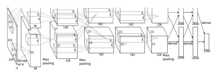
However, there exist examples of CNNs containing multiple “towers”, where convolutional layers are executed in parallel, with reduced communication between the towers. AlexNet is a well known example:

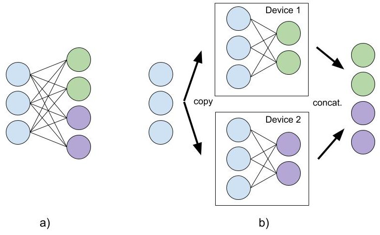
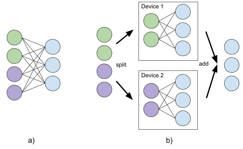
One of the layers best suited to model parallelism is the fully connected or linear layer. Its weight matrix can be split along one dimension or the other, and the resulting submatrices define parallel branches to be executed on multiple devices.

When splitting the weight matrix along the output dimension, the layer in a) is parallelized as shown in b):

When splitting the weight matrix along the input dimension, it looks like this:

This form of parallelism is optimal when the ratio of ratio of activations size to weight size is low (i.e. the weights are relatively large).

Pipelining

Layer partitioning consists in placing a sequence of layers on multiple devices, to be executed as a pipeline.

Pros:

• If a device only computes one operation, weights can remain cached
• Allows to divide weight memory usage. (This is probably the only reason we should consider using layer partitioning.)

Cons:

• Data input rate should match the pipeline execution rate
• Latency is proportional to the number of devices

Pipelining can involve the overlapping of some operations, like computing the forward pass of the current batch and the backward pass of the last batch at the same time. This is why it can sometimes be considered as a form of parallelism. This can be implemented at the framework level, so we probably shouldn’t care about this. This is described in the famous paper “One weird trick for parallelizing convolutional neural networks” (as well as the suggestion to use data parallelism for convolutions and network parallelism for FC layers).