Highlights

This paper shows how meaningful loss function visualizations can illustrate the way loss landscape geometry affects generalization error and trainability. This allowed the authors to explain some known facts about deep neural nets and provide key suggestions for network design and optimization.

Simple loss landscape visualization methods

The authors first describe two well-known methods to visualize a loss function \(L(\theta)\) where \(\theta\) are the weights of a neural network.

1D linear interpolation (1D visualization)

One simple way of visualizaing a loss function is to take two sets of weights \(\theta\) and \(\theta'\), interpolate it

\[\theta(\alpha)=(1-\alpha)\theta+\alpha\theta'\]

and then plot \(L(\theta(\alpha))\) for various values of \(\alpha\) between 0 and 1. This is useful to visualize the ‘'’flatness’’’ of a loss function.

Contour plots (2D visualization)

One can also choose a center point \(\theta^*\) as well as two direction vectors \(\delta\) and \(\eta\) and plot a 2D surface by choosing various positive and negative values of \(\alpha,\beta \in R\):

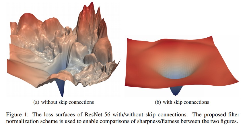
\[L(\theta^*+\alpha\delta+\beta\eta)\]

This typically results into plots such as the ones in Fig.1

Filter normalization for visualization.

Authors mention that one has to take into account the filter weights before to visualize a loss landscape otherwise comparision between different network configurations is impossible. The reasons being that a neural net with large weights may appear to have a smooth and slowly varying loss function. This is problematic considering that with batch norm and relu, one can multiply the weights by a non zero factor and still have the same function.

To remove this scaling effect, they plot the loss using filter-wise normalized directions. Given a random direction \(d\) (which is like \(\delta\) and \(\eta\) above), the elements of \(d\) are normalized as follows:

\[d_{ij} \leftarrow \frac{d_{ij}}{||d_{ij}||} ||\theta_{ij}||\]

where \(i\) is the i-th filter and \(j\) is the j-th layer.

Results

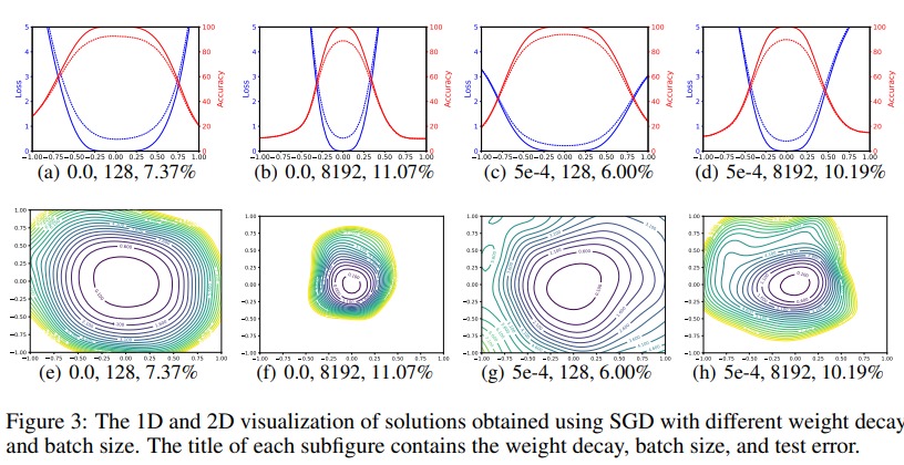
In figure 3, they show the loss landscape around the global minima when using a large and a small batch size with and without weight decay. They come to the conclusion that smaller batch size produces wider minima and lower error rate.

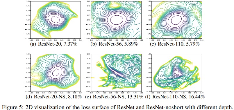
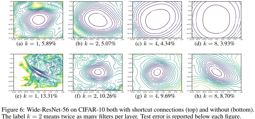
They also show in Fig.1, 5 and 6 that the absence of residual connexion leads to cramped loss landscapes with deep networks.

Conclusion

With this visualization method, the authors came to validate the following statements:

• as networks become very deep, neural loss landscapes go from almost convex to very chaotic. Also, chaotic landscape = poor trainability and large generalization error
• residual connections (ResNet, wideResNet, etc) and skip connections (DenseNet) enforces smooth landscapes
• Sharp loss landscape = large generalization error.
• Flat loss landscape = low generalization error.
• the width of the global minima is inversely proportional to batch size.