Highlights

Authors propose a Vector Quantised-Variational AutoEncoder (VQ-VAE), a variant of VAEs based on two key motivations: (i) discrete variables are potentially better fit to capture the structure of data such as text; and (ii) to prevent the posterior collapse in VAEs that leads to latent variables being ignored when the decoder is too powerful.
Authors introduce a new family of generative models successfully combining the VAE framework with discrete latent representations through a novel parameterisation of the posterior distribution of (discrete) latents given an observation.

Introduction

Discrete representations are potentially a more natural fit for many modalities, such as speech-related tasks.

Most VAE methods are typically evaluated on relatively small datasets such as MNIST, and the dimensionality of the latent distributions is small.

VAEs typically consist of 3 parts:

An encoder network that parameterizes the posterior $$q(z x)$$ over latents
A prior distribution $p(z)$
A decoder with distribution $$p(x z)$$ over input data

Typically the prior and posterior are assumed to be normally distributed with diagonal variance. The encoder is then used to predict the mean and variances of the posterior.

In the proposed work however, authors use discrete latent variables (instead of a continuous normal distribution).

Methods

Authors build upon the regular VAE concept where an input $x$ is generated from a random latent variable $z$ by a decoder $p(x|z)$. Contrary to the standard framework, authors use a discrete latent space, $z \in \mathbb{R}^{K \times D}$, where $K$ is the number of codes in the latent space and $D$ is their dimensionality.

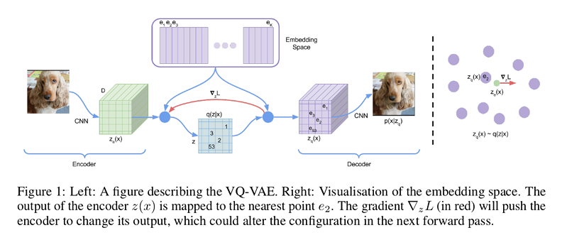
The model takes an input $x$, that is passed through an encoder producing output $z_{e}(x)$. The discrete latent variables $z$ are then calculated by a nearest neighbor look-up using the shared embedding space $e$:

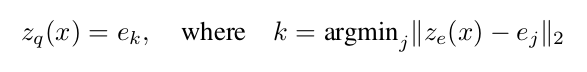
This forward computation pipeline can be seen as a regular autoencoder with a particular non-linearity that maps the latents to 1-of-$K$ embedding vectors.

The posterior and prior distributions are categorical, and the samples drawn from these distributions index an embedding table. Thus:

Encoders model a categorical distribution, sampling from which integral values are obtained
These integral values are used to index a dictionary of embeddings.
The indexed values are then passed on to the decoder.

During forward computation the nearest embedding $z_{q}(x)$ is passed to the decoder.

However, the mapping from $z_{e}$ to $z_{q}$ is not differentiable. In order to alleviate this, authors use a straight-through estimator, meaning that the gradient $\nabla_{z}L$ from the decoder input $z_{q}(x)$ (quantized) are directly copied to the encoder output $z_{e}(x)$ (continuous) during the backward pass.

Therefore, in order to learn the embedding space, authors use a dictionary learning technique, Vector Quantisation (VQ). The VQ objective uses the l2 error to move the make the latent code closer to the continuous vector it was matched to.

Thus, the loss function has three components:

The first term is the reconstruction loss (which optimizes the decoder and the encoder). Since a uniform prior for $z$ is assumed, the KL term that usually appears in the ELBO is constant w.r.t. the encoder parameters and can thus be ignored for training.
The second term is the contribution of the VQ, which optimises the embeddings. sg stands for “stop gradient” and is defined as identity at forward computation time and has zero partial derivatives, constraining its operand to be a non-updated constant.
The third term is a regularization term they name as committment loss which controls the volume of the latent space by forcing the encoder to commit to the latent code it matched with, and avoid its output space growing unboundedly.

The second contribution of this work consists in learning the prior distribution. During the training phase, the prior $p(z)$ is a uniform categorical distribution. After the training is done, they fit an “autoregressive distribution” over the space of latent codes.

Results

Images

Three complex image datasets (CIFAR10, ImageNet, and DeepMind Lab) were used.

The proposed model is compared to the standard continuous VAE framework. It seems to achieve similar sample quality, while taking advantage of the discrete latent space. The model still performs well when using a PixelCNN decoder on top of the VQ-VAE.

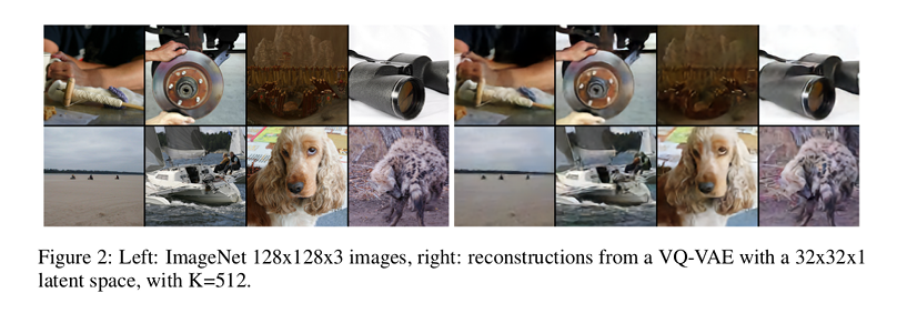
Figure 3 show the images generated by the VQ-VAE using a PixelCNN decoder trained on ImageNet.

Audio

Experiments were done using the VCTK raw speech dataset and are available at: https://avdnoord.github.io/homepage/vqvae/

They carried out experiments on the reconstruction of input clips from the low-dimensionality latent space reconstructions, as well as voice style transfer experiments, among others.

Their model is able to factor speaker-specific information and to learn the same embeddings for the same (high-level) contents.

Video

They used the DeepMind Lab environment to generate sequence of frames given a limited set of sequences. Their results show that the model can generate sequences without any degradation in the visual quality whilst keeping the local geometry correct.

Conclusions

The VQ-VAE encoder network outputs discrete, rather than continuous, codes, and the prior is learned rather than being static.

It is the first discrete latent VAE model that gets similar performance as its continuous counterparts.

Advantages of their method:

It is simple to train.
It does not suffer from large variance.
It avoids the posterior collapse issue which has been problematic with many VAE models that have a powerful decoder, often caused by latents being ignored.

Comments

The learning of the prior over the latent distribution is not clearly explained.