Context-encoding Variational Autoencoder for Unsupervised Anomaly Detection
Highlights
- Novel anomaly detection method, combining a Context Encoder with a Variational Autoencoder, to identify and localize abnormal regions in medical images
- Fuse the deviations from the prior in a Variational Autoencoder with the reconstruction error to improve the localization
- Outperform the state-of-the-art unsupervised approaches on two public segmentation challenges
Introduction
Autoencoder Models
Context Encoders (CEs) are a special class of DAEs where instead of the commonly used additive Gaussian noise local patches of the input are masked out.
Anomaly Detection
There are 3 main groups of methods for unsupervised anomaly detection/localization:
- Classification-based (OC-SVM)
- Reconstruction-based (AE, DAE, CE, VAE)
- Density-based (neighborhood, clustering, VAE)
Classification-based methods can only detect sample-wise anomaly, and cannot be used for localization.
Reconstruction-based methods allow a pixel-wise anomaly detection and can delineate the pathological conditions. However, the reconstruction-error has no formal assertion and no theory-backed validity, rendering it unsuited as a well-calibrated and comparable anomaly score.
Density-based methods allow for a straight-forward normality-scoring and -ordering. However, they often struggle in high dimensional data settings, in addition to not directly giving an anomaly score on a pixel level.
Current anomaly detection methods employ VAEs for reconstruction and still use only the reconstruction-error model for anomaly scoring, thus ignoring an essential part of the model.
Methods
By combining CE and VAE, the authors propose the new Context-encoding Variational Autoencoder (ceVAE), shown in figure 1. The authors claim that they “use the model-internal latent representation deviations and a more expressive reconstruction error for anomaly detection on a sample as well as pixel level.” They also claim that “the denoising task is expected to gear the reconstruction error towards the approximation of the derivative of the log-density with respect to the input.”
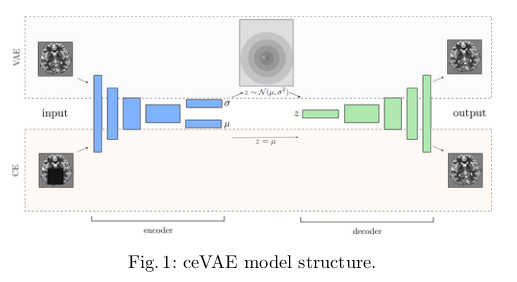
The weights are shared between the CE and VAE, and the CE directly uses the mean of the predicted latent space distribution. Otherwise, the pipeline seems to be standard for autoencoders.
The global loss of the model is a sum of the loss of the CE and VAE, as shown in the equation below:

For the anomaly detection in itself, the density-based score is given by a pixel-wise back-tracing of the latent variable deviations from the prior, which is calculated by back propagating the approximated ELBO onto the input. An element-wise function is used to combine the reconstruction and density scores, as shown in the equation below:
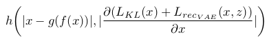
Their claim is that this combination outlines the “direction towards normality” for each pixel.
Data
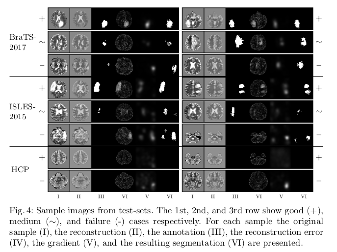
The method was tested on T2-weighted images from three different brain MRI datasets (HCP, BraTS-2017 and ISLES-2015). The HCP dataset, comprised of healthy patients, was the only one used for training. The model was also validated on HCP, and validated and tested on
Results
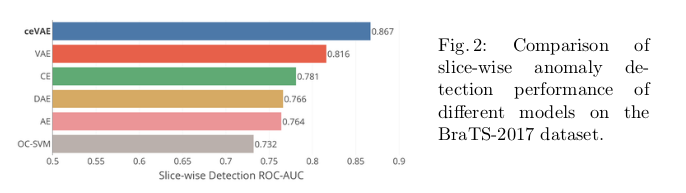
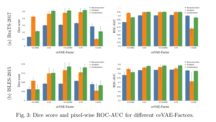
The the slice/sample-wise performance and the pixel-wise performance were evaluated separately.
To explain the low absolute pixel-wise performance seen in Fig. 3, the authors point to “the difference in dataset quality and thus the data distribution to start with.”
Conclusions
The authors mention some still ungoing challenges concerning anomaly localization. They state that “not all anomalies in the dataset might be labeled, thus the performance on those datasets might lower bound the actual performance.” They also point to domain shifts between different datasets obstructing the evaluation.
One particularly interesting area for future research mentionned concerns the VAE sampling. The authors propose that “bigger sampling size for the MC-sampling of the VAE might give insights into areas where the learned data distribution is not well represented and thus indicates anomalies.”
Remarks
The method as it was tested seems to deviate from the proposed theoretical method in one aspect. The authors admit that since back-propagating the \(L_{recVAE}\) showed no additional benefit and only slowed down gradient calculation, they only backpropagate the KL-Loss \(L_{KL}\) to the image.