Highlights

• Replace the RNN hidden state by a finite set of learnable states using a stochastic state transition mechanism
• “Stabilizes” the hidden state for long sequences
• “Better interpretability and explainability”

Method

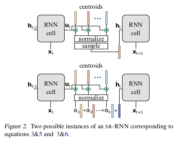
Model figure

Method summary

The hidden state of the RNN is replaced by \(S\), a \(d \times k\) matrix, where \(k\) is the number of possible states (centroids) and \(d\) is the dimension of the hidden states.

A probability distribution is computed using Eq.3, where \(\mathbf u_t \,\) is the “regular” output of an RNN timestep.

Note: The computation is a softmax that uses a temperature parameter \(\tau\), that pushes the distribution towards a one-hot encoding as it decreases.

Then, in theory, a new state is sampled, but this would make the RNN un-differentiable (see top of Fig.2); instead, the new state is a weighted sum of the centroids (see bottom of Fig.2) :

• For memory-less RNNs (such as GRU), it means that they can be represented by a Deterministic Finite Automata as \(\tau \rightarrow 0\).
• For memory RNNs (such as LSTM), it pushes the representational power to the cell state instead of the hidden state.
• In all cases, it limits drifting (where the values of the hidden state increase in magnitude with the length of the sequence).

Experiments

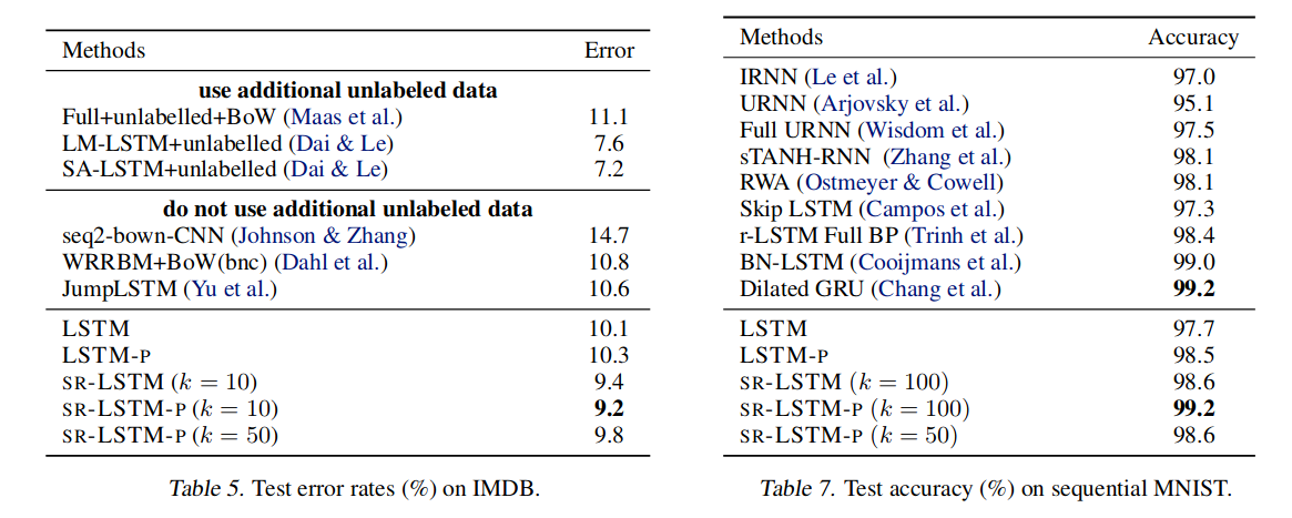
• IMDB (sentiment analysis)
• Sequential MNIST

Results

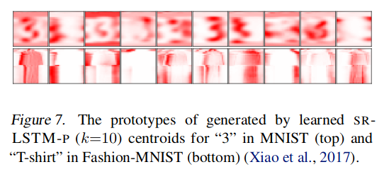
Learned centroids