Striving for Simplicity in Off-policy Deep Reinforcement Learning
Highlights
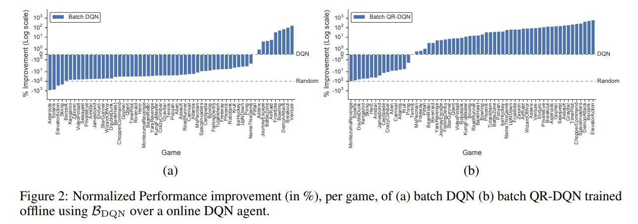
- Learning offline with DQN doesn’t work really well
- QR-DQN and C51 work better in the offline setting than DQN but are complicated
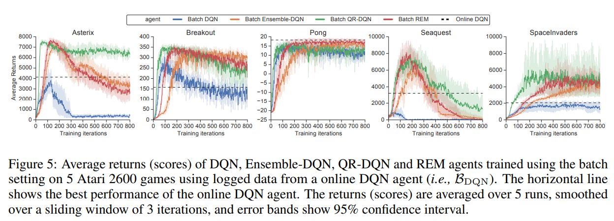
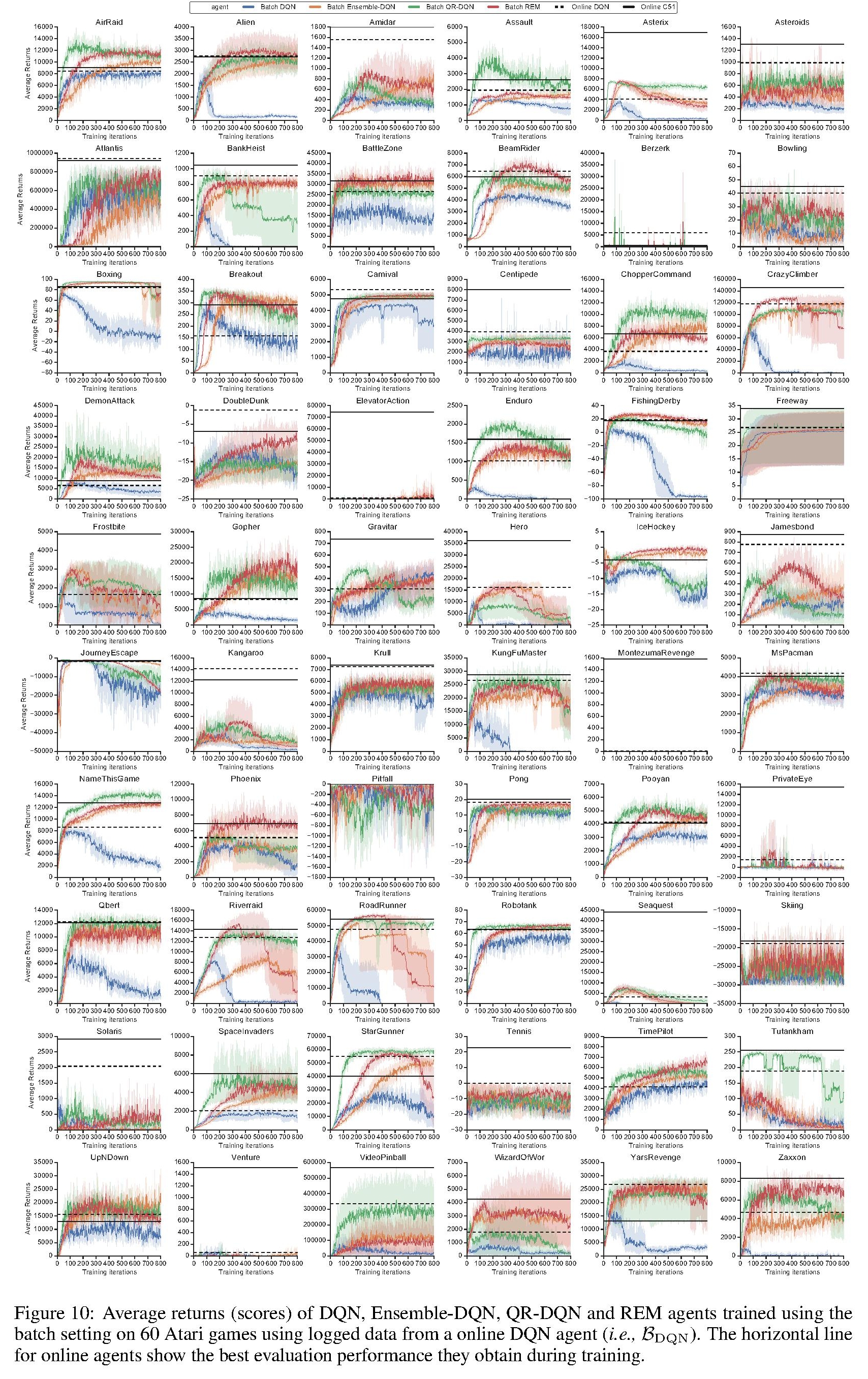
- Ensemble-DQN and REM both outperform DQN and provide similar performance to distributional algorithms in the offline setting
Introduction
Ever since the Nature Deep Q-Network paper, DQNs have been very promising for Deep Reinforcement Learning (DRL). However, their sample efficiency is often criticized; for example, requiring a couple of millions of frames to achieve human-level performance on Atari games. Offline (and off-policy) learning is a way to alleviate this problem by learning on a fixed set of samples collected from any policy.
Q-learning tries to maximize the expected cumulative discounted reward

which can be defined recursively as

with the optimal Q-function defined as

Distributional RL makes use of a distribution over returns \(Z^{*}(s,a)\) instead of the scalar function \(Q^{*}(s,a)\). In this context, the Bellman optimality operator is defined as

with either a categorical distribution supported on a fixed set of locations \(z_{1..k}\) (C51) or a uniform mixture of \(K\) Diracs (QR-DQN). Both are not necessarily offline.
Can Pure Off-Policy Agents Succeed?
The authors first trained a standard Nature DQN and saved every interaction with the environment, which became the dataset \(\mathcal{B}_{DQN}\).
They then trained a DQN agent and a QR-DQN in a batch (offline) setting.
Distilling the Success of Distributional RL into Simpler Algorithms
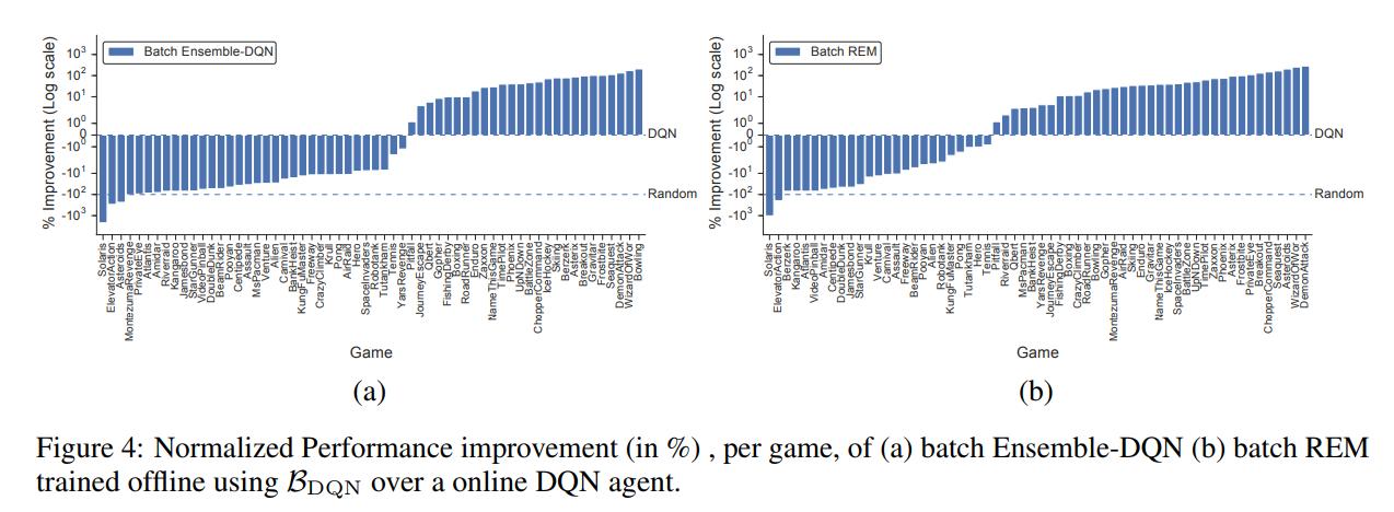
It is still unclear why distributional RL algorithms perform as well as they do. Can simpler algorithms achieve similar results? The authors propose two alternatives: Ensemble-DQN and REM.
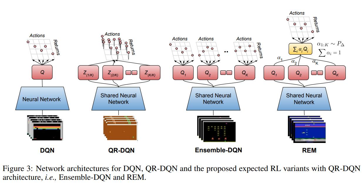
Ensemble-DQN uses an ensemble of Q-heads with a shared network body. The different heads are initialized and trained separately and only the mean of the \(K\) estimates are used as the Q-value.
REM is similar to Ensemble-DQN, but a convex combination of the Q-heads is used as the Q-function. Each head is weighted by \(\alpha_{1..K} ~ P_\Delta\) where \(P_\Delta\) represents a probabiliy distribution over a \(K-1\) simplex \(\Delta^{K-1} = \{\alpha \in \mathbb{R}^{K}: \alpha_1 + \alpha_2 + ... + \alpha_K = 1, \alpha_l \gt 0; k=1..K \}\)
\(\alpha_k\) does not actually change during training and is only sampled from a zero-mean unit-variance gaussian and then normalized. The authors provide proof of why this makes sense in the paper.