Highlights

Authors propose a method named Degenerative Adversarial NeuroImage Net (DaniNet) to Simulate magnetic resonance Imaging (MRI) data representative of neurodegenerative diseases.

Their method uses an adversarially trained autoencoder to capture the patterns that characterize the progression of such diseases. They are also able to condition the generated images on non-imaging features (such as age, diagnosis, etc.).

Introduction

Simulating images representative of neurodegenerative diseases is important for predicting patient outcomes and for validation of computational models of disease progression. Traditional computational methods are limited by imposing a parametric model for atrophy and are extremely resource-demanding.

Other generative models that have been proposed in literature have a few limitations, such as introducing the same morphological changes across all subjects.

Methods

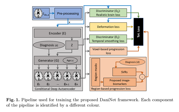
The first pre-processing block (blue) extracts a normalized slice $x$ from the MRI. The second component (grey) is a Conditional Deep Autoencoder (CDA) composed of two deep neural networks: an encoder $E$ that embeds $x$ in a latent space $Z$, and a generator $G$ that projects the vectors produced back to the original manifold.

The latent vector $z$ is conditioned on two variables:

$d$ the diagnosis,
$a \in [1, A]$ the age group, which allows to compute the deformation loss (yellow) to learn morphological changes along the progression.

The output of $G$ are synthetic images defined as $g_{a} = G(E(x), a, d)$.

The third component (green), consists of two discriminator networks:

$D_{z}$ that drives $E$ to produce $z$ with a uniform prior and smooth temporal progression.
$D_{b}$ that drives $G$ to produce realistic brain neuroimages.

Finally, disease progression is modeled through some biological constraints (orange).

Two discriminators are used for the adversarial training:

The first discriminator $D_{z}$ guides $E$ to generate $z$ with a uniform distribution to ensure temporal smoothness:

\[min_{G} max_{D_{z}} \mathbb{E}_{z^{* }} [ \log D_{z} (z^{* })] + \mathbb{E}_{x} [1 - \log D_{z} (E(x))]\]

$z^{* }$ is a vector sampled from $\mathbb{U}$, and $E(x)$ is the latent vector obtained from $x$.

The second discriminator $D_{b}$ guides the generator $G$ to produce realistic brain images:

\[min_{G} max_{D_{b}} \mathbb{E}_{x} [ \log D_{b} (x))] + \mathbb{E}_{x} [1 - D_{b} (G(E(x), a, d))]\]

Three loss functions are used to drive the training: the loss functions $L_{reg}$ and $L_{vox}$ ensure monotonic intensity change to mimic neurodegeneration, and $L_{def}$ together with $D_{b}$ ensure realistic brain morphology.

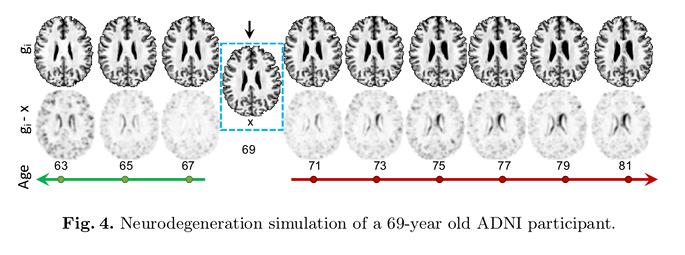
Given a synthetic output $g_{a}$ in age group $a$, authors impose that the corresponding voxels of each preceding image $g_{i}$ with $i < a$ have higher-intensity values. Likewise, later images $g_{j} with$j > a$$ have lower-intensity values:

\[L_{vox}= \frac{1}{MN(A - 1)} \left[ \sum_{p=1}^{a-1} sgn(g_{a} - g_{p}) + \sum_{p=a+1}^{A} sgn(g_{p} - g_{a}) \right]\]

where $g_{i}$ (with $i \in [1, A]$) is the image sequence.

Authors use another term to improve spatial consistency across neighboring voxels. This terms operates at a regional level. Pre-trained SVRs are used to supply a set of constraints on the generator’s outputs for ensuring accurate emulation of neurodegeneration:

\[L_{reg} = \frac{1}{R(A - 1)} \sum_{i=1}^{R} \left[ \sum_{p=1}^{a-1} \left( SVR_{i}(p, a, d) - \frac{\sum[g_{a} \cdot r_{i}] + \epsilon}{\sum[g_{p} \cdot r_{i}] + \epsilon} \right) + \\ \sum_{p=a+1}^{A} \left( SVR_{i}(p, a, d) - \frac{\sum[g_{p} \cdot r_{i}] + \epsilon}{\sum[g_{a} \cdot r_{i}] + \epsilon} \right) \right]\]

where $R$ is the number of regions, $r_{i}$ is the $i$-th region-mask, $SVR_{i}(p, a, d)$ is the prediction of intensity rate progression for the region $i$, and $\epsilon = 0.1$ avoids division by 0.

The deformation loss minimises the difference between each input image $x$ and a weighted average of two outputs from the nearest age bins:

\[L_{def} = L_{2} \left( x, [g_{a} \alpha + g_{a + 1} (1 - \alpha)] \right)\]

where $\alpha$ reflects the distance between input age and the group $a$ and $a + 1$.

Data

Authors used T1-weighed longitudinal MRI images from the ADNI dataset to train and test their method:

9652 images (876 subjects) for training.
1283 images (179 subjects) for testing.

Pre-processing consists of linear co-registration to the MNI template, skull-stripping, and intensity normalization.

Results

In the figures below $x$ indicate baseline visits, and $y$ corresponds to follow-up visits (ground-truth). Results are reported as different combinations of the proposed loss functions/priors:

$P$ obtained exploiting $L_{vox}$ and $L_{reg}$.
$C$ obtained conditioning the system with the clinical diagnosis.
$T$ obtained when the learned model is transferred before testing on new data.

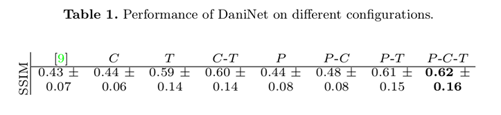
Quantitative comparison between images $y$ and predicted images is done using Structural Similarity Index Matrices (SSIM).

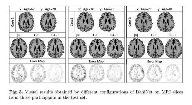
Qualitative comparisons were also carried out to assess the perception of medical imaging experts by asking to select the closest synthetic image from the pool of configurations.

Clearly, the best results are obtained when the framework includes all three components. The baseline model produces inferior SSIM. Transfer learning $T$ is the feature that provides the highest contribution.

Conclusions

Authors experiments demonstrate that their proposed method shows the ability to produce accurate and realistic synthetic MRI images that emulate neurodegenerative disease progression.