Highlights

• A loss prediction module that can be used to select the next data points to be labeled based on the highest-loss in an active-learning context

Introduction

In an active-learning context, only a small subset of the dataset is labeled. Then, some data points are selected to be labeled and used during training. The task of selecting which points should be selected is still an open problem. The authors propose selecting the data points which should incur the highest loss during training. To find these points, the authors propose training a smaller network that can predict the training loss.

Methods

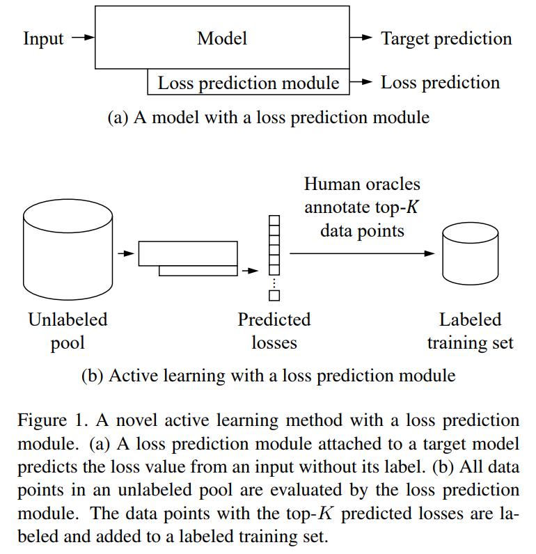
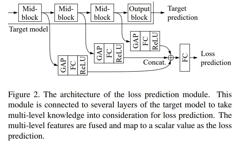
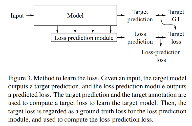
Figure 1,2,3 describe most of the method.

The training process goes like this: First, a subset of the dataset is selected and labeled. Then, both networks are trained. After the training iteration is done, all data points in the unlabelled pool are fed to the loss-prediction network and the top-K points are selected to be added to the labelled set and used for training.

Since the loss-prediction module is fed from the target network, a joint loss function must be used to train both networks:

\[L = L_{target}(\hat{y},y) + \lambda L_{loss}(\hat{l},l)\]

whereas \(\hat{l}\) is the loss of the loss-prediction network and \(l\) is the loss of the target network.

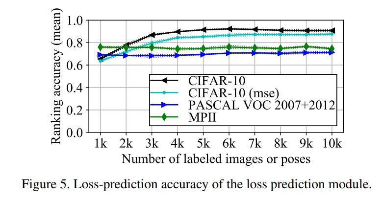
The authors mentioned that they first tried MSE for \(L_{loss}\), however it did not give good results, because, as they theorize, the scale of \(l\) changes over time (since the loss should decrease during training). They therefore propose to compare pairs of samples in the same minibatch, as they should have the same loss scale.

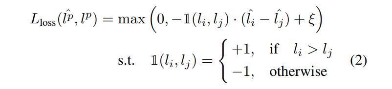
where the supscript \(p\) denotes a pair of data points, \(i, j\) the elements of the pair, \(\xi\) a positive margin. A given example is if \(l_i > l_j\) and \(\hat{l_i} > \hat{l_j} + \xi\), then no loss is given. Otherwise, the loss forces the model to increase \(\hat{l_i}\) and decrease \(\hat{l_j}\).

The final combined loss then becomes:

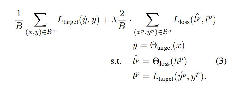
where \(B\) the size of \(\mathcal{B}^s\), the minibatch at the active learning stage \(s\), \(\Theta\) the networks.

Data

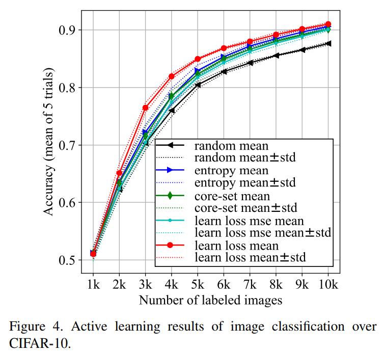
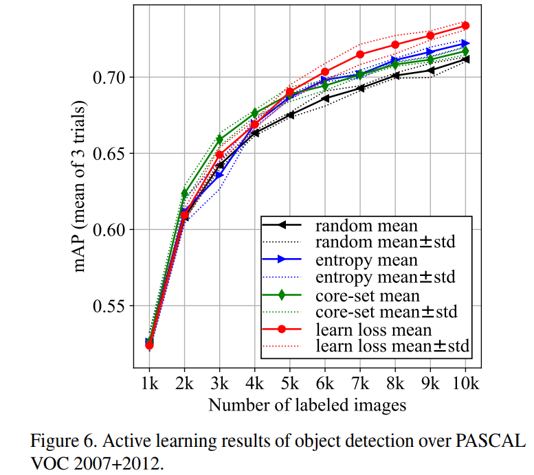
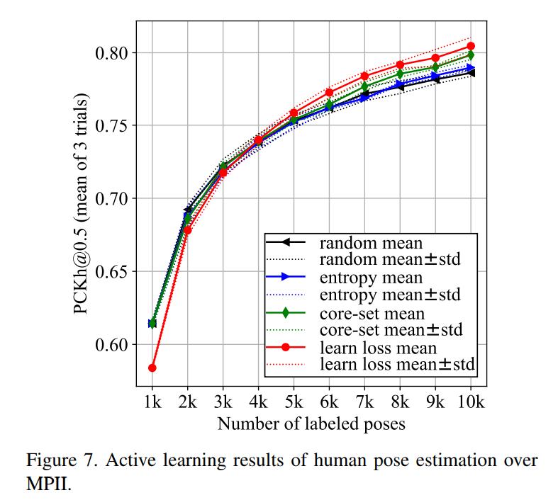
To prove that their method is agnostic to the underlying task, the authors tested their method on three diverse visual recognition tasks: Image classification on CIFAR-10, pose estimation on MPII and object detection on PASCAL VOC 2007 and 2012.

Different models have been used for different tasks.

Results

Conclusions

The proposed method seems to improve on current sampling strategies.

Remarks

Although not by much.