Residual Policy Learning
Highlights
- RPL improves on initial policies
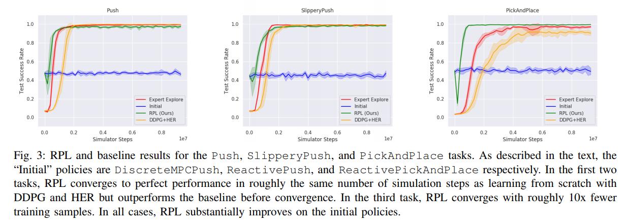
- RPL is more data-efficient than learning from scratch
Introduction
For most complex problems of interest, learning from scratch remains intractable, especially in long-horizon sparse-reward environments. Often, it is easier to provide a hand-crafted policy or a model-predictive controller in the case of robotics. But, these policies are often barely good enough and don’t do well in hard-to-model environments (involving friction for example) or environments full of obstacles.
In this work, the authors propose Residual Policy Learning (RPL), a method for improving existing policies.
Methods

The main idea is to learn to augment existing policies by learning residuals on top of them. Given a policy \(\pi:S \rightarrow A\), the authors propose to learn a residual function \(f_\theta(s):S \rightarrow A\) given by
\[\pi_\theta(s) = \pi(s) + f_\theta(s)\]Because the policy \(\pi\) is fixed, the gradient of the policy \(\pi_\theta\) is given by:
\[\nabla_{\theta}\pi_{\theta}(s) = \nabla_{\theta}f_{\theta}(s)\]Therefore, RPL can be used to improve on non-differentiable policies.
To use these two policies together, let’s remind ourselves that the policy \(\pi\) acts in the Markov Decision Process (MDP) \(M = (S,A, R, T, \gamma)\) where \(S\) is the set of all possible states, \(A\) the set of all possible actions, \(R\) the reward for taking action \(a \in A\) at \(s \in S\), \(T(s, a, s')\) the transition probabilities and \(\gamma\) the discount factor.
The residual policy \(f_\theta\) then acts in the residual MDP \(M^{(\pi)} = (S,A, R, T^{(\pi)}, \gamma)\) where
\[T^{(\pi)}(s, a, s') = T(s, \pi(s)+a,s')\]Thus, standard reinforcement learning can be used to learn the residual policy.

Initializing the residuals
One thing to make sure is that the residuals don’t make the initial policy worse. If the initial policy is perfect, the residuals should have no influence. To alleviate this problem, the authors initialize the residual function so that \(f_{\theta}(s) = 0\) by making the weights of the last layer of their network all zero.
RPL with Actor-Critic Methods
In the case of Actor-Critic methods, because the gradient of the actor depends on the critic, a bad critic may make the actor worse. The authors, therefore, propose to train the critic alone first until its loss dips below a threshold \(\beta\), which they fixed at \(\beta = 1.0\)
Data
Six tasks were tested for this method:
- Push, where the objective is to push an object to a target location
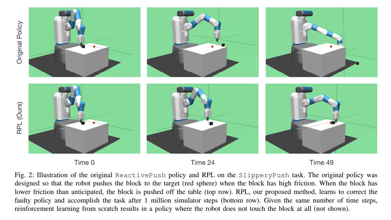
- SlipperyPush, where the goal is still to push an object to a target location, but the object now has less sliding friction with the table
- PickAndPlace, where the target location may now be on the table or above it
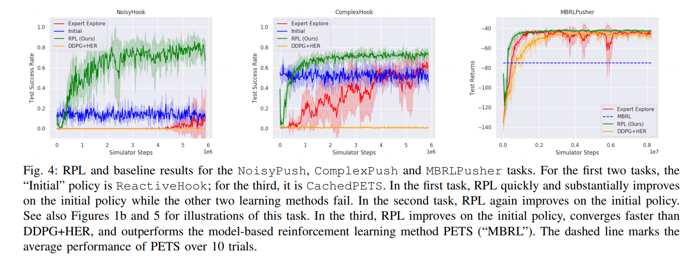
- NoisyHook, where the gripper has to use a hook to move an object to a target location. The Noisy part comes from the observations, which are now gaussian instead of deterministic.
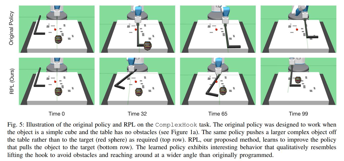
- ComplexHook, where there is no longer observation noise, but the object can be of any shape and there are bumps on the table
- MBRLPusher, where the goal is for a 7-DOF robot to push a cylinder to a target.
Various initial policies, whether model-predictive controllers or reactive policies, were used for different tasks.
Results


Conclusions
RPL consistently improves on initial policies and achieves better data efficiency and performance than model-free RL alone.