Batch Policy Gradient Methods for Improving Neural Conversation Models
Highlights
- Off-policy offline (batch) training for policy-gradient algorithms using LSTMs
Introduction
In this paper, the authors study the use of off-policy offline learning with Seq2Seq recurrent neural networks architectures to improve conversational agents.
Policy gradient: A lot of deep learning approaches to reinforcement learning (RL) make use of Q-learning, where the goal is to estimate the optimal action value function \(Q^*\) and then to choose the action that greedily maximizes \(Q^*\). However, estimating \(Q^*\) in large action spaces can be quite challenging. Policy gradient methods instead make changes to the parameters of a policy along the gradient of a desired objective.
Off-policy vs. on-policy: On-policy methods referer to improving the current policy on the fly while exploring the environment. Off-policy methods refer to using a behavioral policy to navigate in the environment while improving a different policy.
Online vs offline learning: Online learning refers to the policy interacting with the environment. Offline refers to a policy learning from past explorations. Online learning can be done off or on-policy, but offline learning is necessarily off-policy.
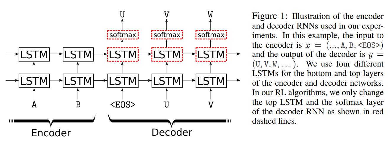
Seq2Seq models: The goal of Seq2Seq models in natural language processing (NLP) is to produce an output sequence \(y = [a_0, a_1, ...a_T]\) from an input sequence \(x\), where \(a_i \in A\) where \(A\) is a vocabulary of words. Typically, an encoder will represent the input sequence as an Euclidean vector and a decoder will convert the vector into an output sequence. In an RL setting, the state at time \(t\) will be the input sequence \(x\) and the actions \(y_{t-1} = [a_0, a_1, ..., a_{T-1}]\)
Methods
The goal is to maximize the following (1):
\[J(\theta) = \sum_{s \in S} q(s)V^{\pi_\theta}(s)\]where \(q\) is the distribution of states. The policy is updated by taking steps along the gradient of the objective,
\[{\nabla}J(\theta) = {\nabla}E_{s~q}[\sum_{a \in A}\pi_\theta(a|s)Q^{\pi_\theta}(s,a)] = E_{s~q}[\sum_{a \in A} \nabla\pi_\theta(a|s)Q^{\pi_\theta}(s,a) + \pi_\theta(a|s)\nabla Q^\pi_\theta(s,a)]\]Because the second term in the above gradient is hardly tractable, it can be ignored and the gradient can be approximated to:
\[g(\theta) = E_{s~q}[\sum_{a\in A}\nabla\pi_\theta(a|s)Q^{\pi_\theta}(s,a)]\]Expanding on \(g(\theta)\), we get:
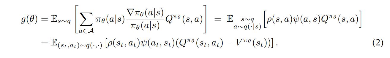
with \(\psi(a,s)=\frac{\nabla_{\pi_{\theta}}(a|s)}{\pi_\theta(a|s)} = {\nabla}log\pi_\theta(a|s)\) the score function of the policy, \(\rho(s,a)=\frac{\pi_\theta(a|s)}{q(a|s)}\) the importance sampling coefficient
The value function \(V^{\pi_\theta}\) was introduced to reduce variance during the SGD updates: If \(Q^{\pi_\theta}(s_t,a_t)\) is large relatively to \(V^{\pi_\theta}(s_t)\), the coefficient of the score function will influence changes to \(\theta\) to assign a higher probability to \(a_t\) at \(s_t\)
However, \(Q^{\pi_\theta}\) and \(V^{\pi_\theta}\) aren’t available. \(Q^{\pi_\theta}(s_t,a_t)\) can be approximated by summing the future rewards at the current state. However, since trajectories come from \(q\) and not \(\pi_\theta\), the authors use \(\lambda-return\), a convex combination of the re-weighted rewards defined recursively from the end as

\(V^{\pi_\theta}\) still needs to be defined. Approximating it can be quite difficult as \(S\) can be potentially infinite. However, the role of \(V\) is only to reduce variance and does not need to be exact or even precise. Two options are proposed to approximate \(V\): The first one being a constant equal to the mean reward of the entire dataset. The second option uses the parametrisation \(V(s)=\sigma(\xi^T\phi(s))\) estimated using the \(GTD(\lambda)\) estimator. Their implementation of it is available in the appendix of the paper.
With \(Q^{\pi_\theta}\) estimated as \(r^{\lambda}_{t}\) and \(V^{\pi_\theta}\) estimated as \(\hat{V}\), the update rule for the parameters of the policy can be defined as

and the algorithm for Batch PG as
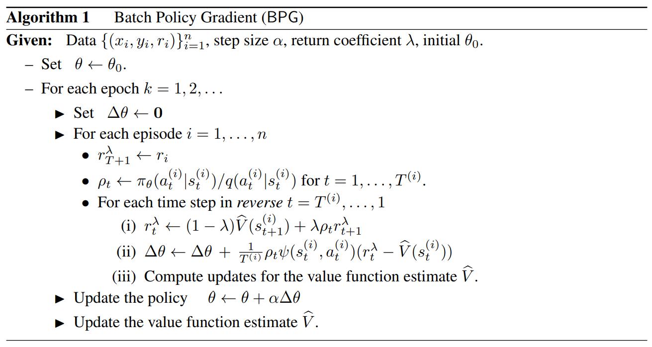
In a less mathematical manner, the model used is a two-layer LSTM where only the top layer of the decoder part is updated:
Data
The authors first tested on the Europarl Dataset where the goal is to reproduce the input sequence without using some forbidden words.
Results
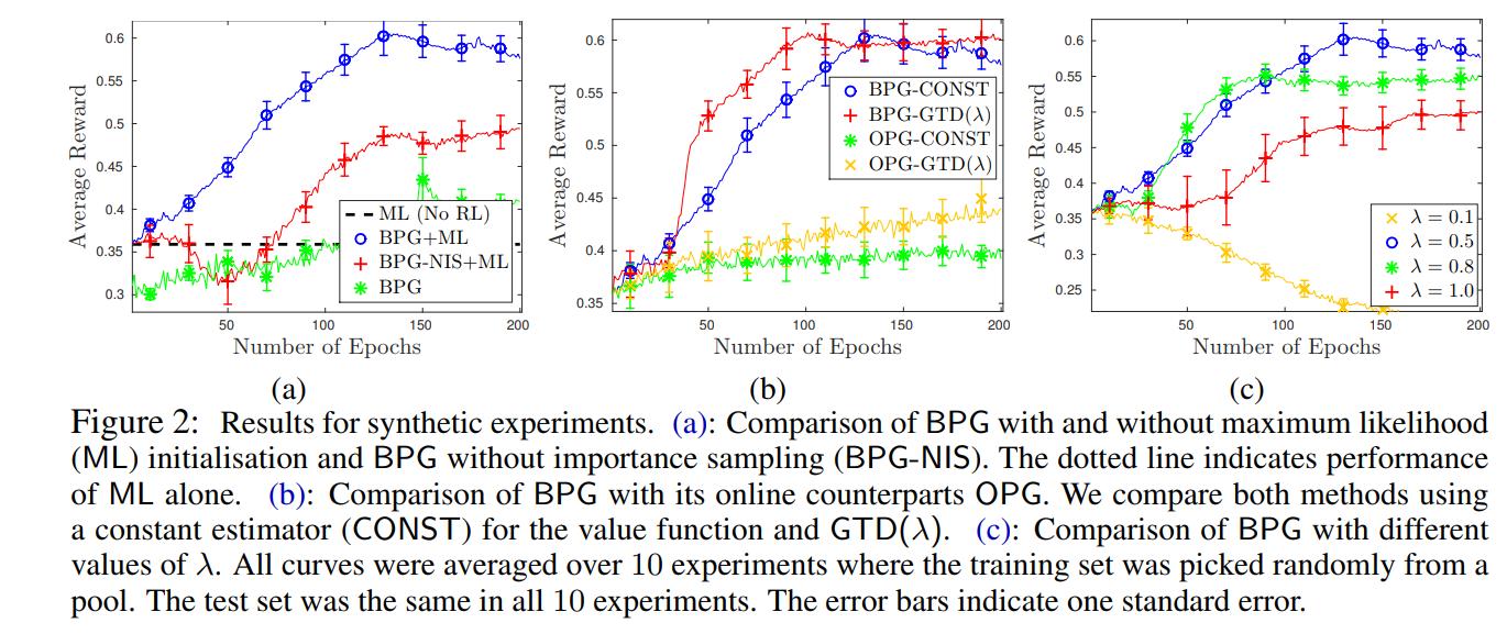
The authors then validated their experiments on an online restaurant recommendation service. The authors first trained the model via supervised maximum likelihood on 6000 conversations of this dataset, and then generated 1216 responses from these conversations and had them ranked 0-2 which served as the reward for these responses.
The authors then trained their model on this dataset using BPG and BPG+ML bootstrapping and tested on 500 separate conversations, which were then also ranked 0-2. The results are below:
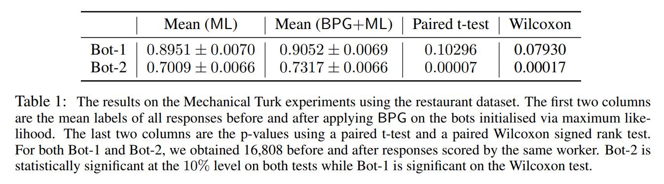
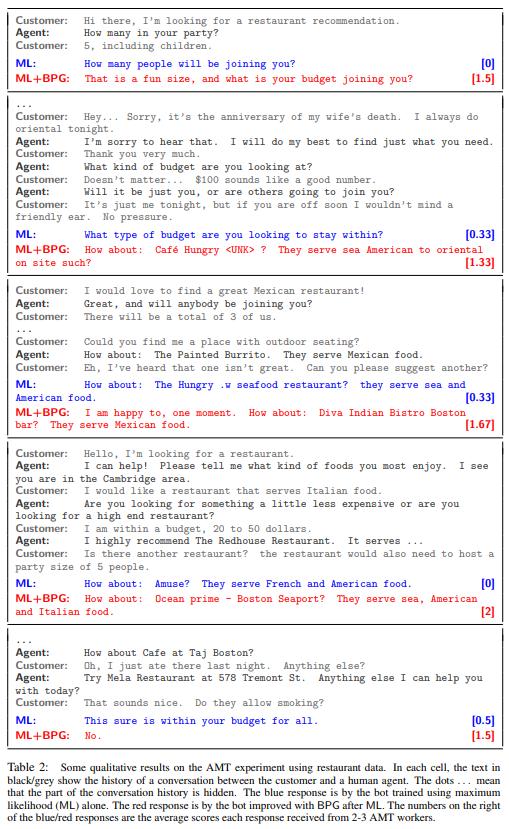
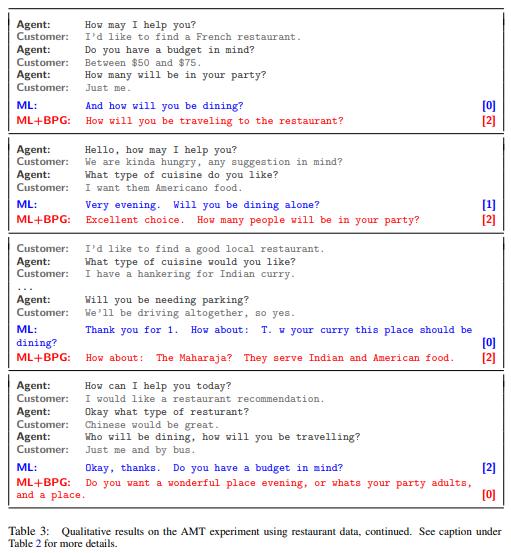
and some qualitative results:
Conclusions
The proposed method works really well when you have a lot of unlabelled data and some expensive-to-acquire labelled data, and works marginally better than solely supervised learning.