The active learning setting works with a large unlabeled dataset, that is labeled progressively by an oracle, according to the selections of the active learning method. The data points to be labeled are selected using an acquisition function, that takes an image as input and outputs a value that represents how useful the label would be. The best active learning method achieves the highest accuracy with the fewest labeled data points. In this paper, multiple active learning methods are studied.

Methods

Uncertainty estimation

The most successful acquisition functions are uncertainty based: they work on a probability distribution on the classes (a “softmax vector”). The softmax output of a single network is generally not a good uncertainty measure, but taking the average of multiple of those vectors is better. The authors consider two approaches for producing multiple softmax predictions:

Monte-Carlo Dropout
T forwards passes are executed on a network, each with different dropout masks; the T resulting softmax outputs are averaged. In this work, T=25.
Ensemble
N identical networks are trained with different random seeds. The softmax output of the N networks are averaged. In this work, N=5.

Acquisition functions

The authors consider two types of acquisition functions: uncertainty based and density based. The second type underperforms and thus will not be described here.

Entropy
Choose the points for which their softmax output have the highest entropy.
Mutual information between data-points and weights
Choose the points for which the mutual information is the highest. The idea is that a large mutual information between a prediction and the weights means that obtaining the ground truth and training on it would have a large impact on the weights.
Variation ratio
Choose the points that have the hight variation ratio. The variation ratio is the proportion of predicted class labels that are not the modal class prediction. Suppose that an ensemble produces the following class predictions: [4, 1, 4, 4, 3]. In this example, the variation ratio is 2/5, because two networks have given a different prediction than the modal prediction (4).
Random
This is used as a control and should be equivalent to non-active learning.

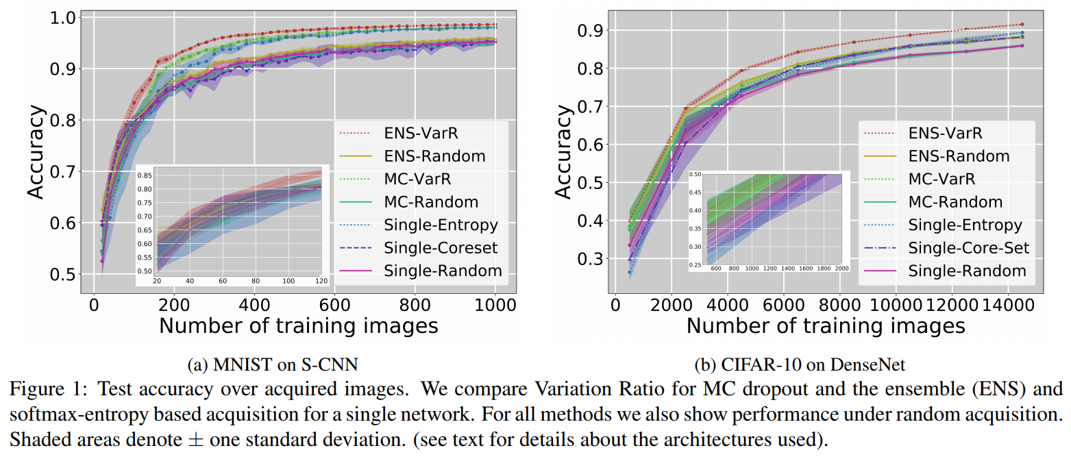
Main results

Notes on the naming convention in the legends:

The uncertainty estimation method (ENS, MC, Single) is followed by the acquisition function (VarR, Random, Entropy, Coreset).
“VarR” means Variation Ratio.
“Single” is an “ensemble” of size 1.
“Coreset” is a density-based method.

Other results are provided, including a study on the size of the ensembles, and ways to make ensembling less computationally expensive.

Conclusion

In this study, the combination of using an ensemble and the Variation Ratio outperformed the other approaches.