[Contrastive Loss] Dimensionality Reduction by Learning an Invariant Mapping

Summary

The contrastive loss proposed in this work is a distance-based loss as opposed to more conventional error-prediction losses. This loss is used to learn embeddings in which two “similar” points have a low Euclidean distance and two “dissimilar” points have a large Euclidean distance.

While this is one of the earliest of the contrastive losses, this is not the only one.¹ For instance, the contrastive loss used in SimCLR is quite different.

Proposed method

Two samples are either similar or dissimilar. This binary similarity can be determined using several approaches:

• In this work, the N closest neighbors of a sample in input space (e.g. pixel space) are considered similar; all others are considered dissimilar. (This approach yields a smooth latent space; e.g. the latent vectors for two similar views of an object are close)
• To the group of similar samples to a sample, we can add transformed versions of the sample (e.g. using data augmentation). This allows the latent space to be invariant to one or more transformations.
• We can use a manually obtained label determining if two samples are similar. (For example, we could use the class label. However, there can be cases where two samples from the same class are relatively dissimilar, or where two samples from different classes are relatively similar. Using classes alone does not encourage a smooth latent space.)

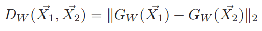
Formally, if we consider \(\vec X\) as the input data and \(G_W(\vec X)\) the output of a neural network, the inter-point distance is given by

The contrastive loss is simply

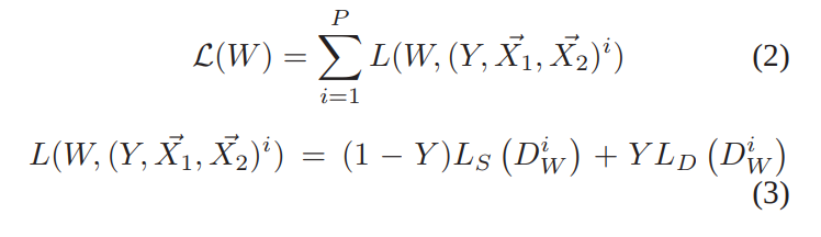
where \(Y=0\) when \(X_1\) and \(X_2\) are similar and \(Y=1\) otherwise, and \(L_S\) is a loss for similar points and \(L_D\) is a loss for dissimilar points. More formally, the contrastive loss is given by

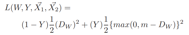
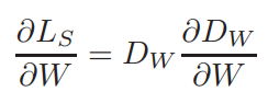
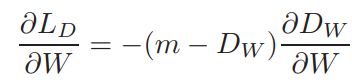
where $m$ is a predefined margin. The gradient is given by the simple equations:

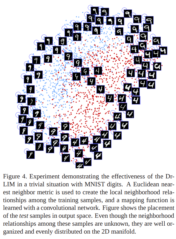
Results

Results are quite convincing.

Blog

A nice blog on the contrastive loss (and other losses).

References