Improved Image Captioning via Policy Gradient optimization of SPIDEr
Introduction
Image captioning trained with maximum likelihood estimation often does not correlate with human assessment of quality. Evaluation metrics such as SPICE and CIDER offer a better evaluation of image captioning quality. However, these metrics cannot be used with maximum likelihood estimation as they are not differentiable. The authors of this paper propose a new technique using policy gradient to train on these metrics. This method is an improvement over the MIXER technique (https://arxiv.org/pdf/1511.06732.pdf).
Previous methods
Maximum likelihood
Standard maximum likelihood training where the goal is to maximize the probability of obtaining the ground truth.
\[L(\theta) = \frac{1}{N} \sum\limits^{N}_{n=1} log p(y_t^n|y_{1:t-1}^n, x^n, \theta)\]Mixer
The MIXER paper proposes a method that mixes MLE and REINFORCE. They evaluate the first M words with MLE and the next words with REINFORCE. They gradually decrease M during training until it reaches 0. This method happens to be very sensitive to hyper-parameters.
Method
At time step t an action is chosen. Each action corresponds to a word \(g_t \in V\)(vocabulary). The action is chosen with a stochastic policy \(\pi_\theta(g_t|s_t, x)\). The transition function is deterministic: each word id appended: \(s_{t+1} = s_t:g_t\).
At the end of each sequence (when the end token action is chosen), a reward \(R(g_{1:T}|x^n, y^n)\) is given. This represents the score given by sequence \(g_{1:t}\) given image \(x^n\) and ground truth \(y^n\). The reward can be any function (BCMR, SPICE, CIDER…).
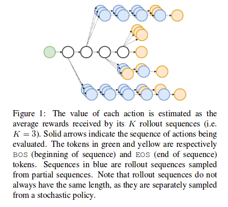
To ensure the agent gets a reward at each timestep K Monte-Carlo rollouts are performed at each step.
The value function for a specific state(sequence) is defined by:
\[V_\theta(g_{1:t}|x^n, y^n) = E_{g_{t+1|T} \sim \pi_\theta(\cdot|g_{1:t}, x^n)} [R(g_{1:t};g_{t+1:T}|x^n, y^n)]\]The goal of the method is to maximize the value function of the first state \(s_0\).
\[J(\theta) = \frac{1}{N} \sum\limits_{n=1}^N V_\theta(s_0|x^n, y^n)\]To maximise this they use:
\[\nabla_\theta V_\theta(s_0) = E_{g_{1:T}}[ \sum\limits_{t=1}^T \sum\limits_{g_t \in v} \nabla_\theta \pi_\theta(g_t|g_{1:t-1})Q_\theta(g_{1:t-1}, g_t) ]\]Where: \(Q_\theta(g_{1:t-1}, g_t) = E_{g_{t+1:T}}[ R(g_{1:t-1};g_t:g_{t+1:T}) ]\)
The gradient is approximated by sampling M paths from \(\pi_theta\).
\[\nabla_\theta V_\theta(s_0) \approx \frac{1}{M} \sum\limits_{m=1}^M \sum\limits_{t=1}^T E_{g_t}[ \nabla_\theta \pi_\theta(g_t|g^m_{1:t-1})Q_\theta(g^m_{1:t-1}, g_t) ]\]Where the log trick is used and:
\[g_t \sim \pi_\theta(g_t|g^m_{1:t-1})\]In this paper, a value of M = 1 is used.
The Q function is evaluated using K monte Carlo rollouts. K sequences are sampled from the current point and the average is computed.
\[Q(g_{1:t-1}, g_t) \approx \frac{1}{K} \sum\limits_{k=1}^K R(g_{1:t-1};g_t;g^k_{t+1:T})\]This allows for an unbiased but very high variance estimator. In order to reduce the variance, a baseline is used. The baseline is a MLP with parameters \(\phi\) connected to the hidden state of the RNN.
\[B_\phi(g_{1:t-1}) = E_{g_t}[Q(g_{1:t-1}, g_t)]\]The baseline is subtracted from \(Q_\theta\).
The gradient for \(V_\theta(s_0)\) is therefore:
\[\nabla_\theta V_\theta(s_0) \approx \frac{1}{M} \sum\limits_{m=1}^M \sum\limits_{t=1}^T E_t[ \nabla_\theta \pi_\theta(g_t|g^m_{1:t-1})Q_\theta(s_t, g_t) - B_\phi(s_t)]\]where \(s_t = g_{1:t-1}\)
The baseline is trained with the following loss function:
\[L_\phi = \sum\limits_t E_{s_t}E_{g_t}(Q_\theta(s_t, g_t) - B_\phi(s_t))^2\]The baseline’s gradient is not back-propagated through the RNN to avoid a feedback loop.
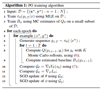
The algorithm to train the network is as follows. In order to prevent the agent from being “too” random, the network is initially trained with MLE before switching to policy gradient.
Architecture
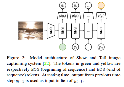
The architecture used is an encoder-decoder. The encoder is an Inception-V3 pretrained on ImageNet and the decoder is a one-layer LSTM with a state size of 512.
Results
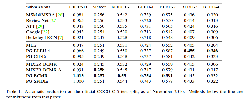
The method was trained to optimize different combinations of metrics, including BCMR (BLEU, METEOR, ROUGE, CIDEr), SPICE and their new metric SPIDEr.
SPICE uses a graph to compare the ground truth and generated sentences. However, it often syntactically wrong. Therefore, the best results were obtained using a linear combination of CIDEr and SPICE, known as SPIDEr.