This paper presents a novel statistical distribution: a CONtinuous relaxation of a disCRETE distribution. Contrary to discrete random variables, the Concrete random variables are suited for use in stochastic computation graphs trained with automatic differentiation.

This is useful for learning the shape of a discrete distribution. The binary case is the Binary Concrete, and is useful, among other things, for pruning a neural network¹.

Discrete Random Variables in a computation graph

Consider \(\mathrm{Discrete}(\alpha)\), a discrete distribution with unnormalized parameters \(\alpha_k \in (0,\infty)\), where the probability of outcome \(k\) is \(\alpha_k / \sum_i \alpha_i\). The sampling from this distribution can be formulated with the Gumbel-Max trick, as seen in Figure 1(a). Note that the discrete values are encoded in a one-hot vector, and that \(G_i\) are samples from the standard Gumbel distribution.

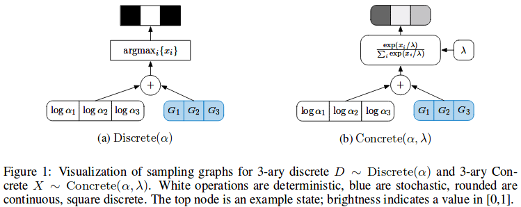
Note that instead of optimizing \(\alpha\) directly, we would optimize \(\log \alpha \in \mathbb{R}\). This allows to avoid constraining the parameters of the network.

Sampling from the standard Gumbel can be done using \(f(U)=-\log(-\log U)\) with \(U \sim \mathcal{U}(0,1)\).

Concrete Random Variables

The derivative of the argmax is 0 everywhere except at the boundary of state changes, where it is undefined. For this reason the Gumbel-Max trick is not a suitable reparameterization for use in stochastic computation graphs trained with automatic differentiation. This is why the Concrete distribution is introduced; see Figure 1(b) for how to sample from it. Basically, the argmax operation is replaced with a softmax.

This allows to optimize \(\alpha_k\) via gradients, and thus learn the shape of the distribution.

The parameter \(\lambda\) acts as a temperature parameter for the softmax; it controls the relaxation. When \(\lambda \to 0\), the softmax becomes an argmax.

The Binary Special Case

Suppose that you want to learn the value of a binary variable, such as the elements of a binary mask. For example, you could want to mask feature maps in a network and find which features to keep or discard.

While a one-hot vector is the standard way of encoding a discrete variable with more than two values, for a binary variable we only need a binary scalar.

Sampling from the Binary Concrete can be done using \(f(U)=\mathrm{Sigmoid}(( \log \alpha + L(U) ) / \lambda)\), where \(L(U)=\log U - \log(1-U),\ U \sim \mathcal{U}(0,1)\) samples from the Logistic distribution. Notice how similar this is to the non-binary case; instead of Gumbel samples, we use Logistic samples, and instead of a Softmax, we use a Sigmoid, but the rest is identical.

Cheat sheet

Distribution	Sampling function
Concrete	\(f(U)=\mathrm{Softmax}((\log \alpha + G(U))/\lambda)\)
Binary Concrete	\(f(U)=\mathrm{Sigmoid}(( \log \alpha + L(U) ) / \lambda)\)
Standard Gumbel	\(G(U)=-\log(-\log U),\ U \sim \mathcal{U}(0,1)\)
Logistic	\(L(U)=\log U - \log(1-U),\ U \sim \mathcal{U}(0,1)\)

Implementation notes

• Optimize \(\log \alpha\) instead of \(\alpha\). I suggest naming your optimized tensor log_alpha.
• Initialize \(\log \alpha\) values around zero. The zero-centered normal with scale \(0.01\) should work.
• Try \(\lambda=2/3\) (see paper for details).

---

Notes