Budget-Aware Regularization (BAR) allows to simultaneously train and prune a neural network architecture, while respecting a neuron budget. The method is targeted at “turning off” irrelevant feature maps in CNNs. To find which feature maps are relevant, “Dropout Sparsity Learning” is used. To respect the budget, a novel barrier function is introduced.

Contributions at a glance:

• Objective function that optimizes/constrains the total number of neurons
• Novel barrier optimization method
• Mixed-Connectivity Block that leverages atypical connectivity

Dropout Sparsity Learning

We learn which feature maps to keep by using a special kind of dropout. The first difference with traditional dropout is that each feature map is associated with a different Bernoulli parametrization (e.g. probability of being active). Let’s call this “feature-wise dropout”.

\(\mathbf{z}\) is a vector of “dropout variables”. The goal is to learn the parametrization of each dropout variable, with a preference for parameterizations that turn off the feature map. However, ordinary feature-wise dropout, because of its discrete nature, does not allow to learn the parameters by backpropagation. We will thus use a continuous relaxation of Bernoulli, named the Hard Concrete distribution. Using the Reparametrization Trick, we can draw samples from the distribution like so:

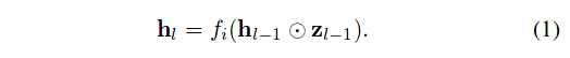
\[\begin{aligned} z &= g(\Phi_{l-1},\epsilon) \\ z &\in [0,1] \\ \epsilon &\sim \mathcal{U}(0,1) \end{aligned}\]

We rewrite Eq. (1) like this:

The following is a plot of the function \(g(\Phi,\epsilon)\) associated with the Hard Concrete. For our purposes, \(\Phi := \alpha\).

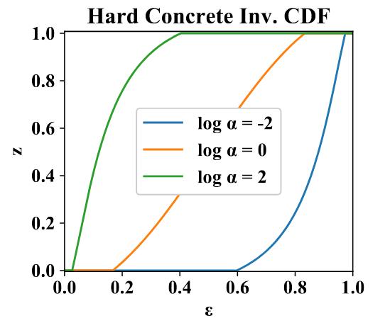
Here is an intuition about this plot. Take the blue curve; it is associated to a irrelevant feature map. Why? Imagine you draw samples \(\epsilon \sim \mathcal{U}(0,1)\) and you give them to this function. It will mostly output zero; in fact \(P(z=0) \approx 0.6\).

The interpretation of \(\alpha\) is that it controls \(P(z=0)\), \(P(z=1)\), and the probability density in between (for \(z \in~]0,1[~\)). The weird thing with the Hard Concrete, is that while there is virtually no chance of picking a specific value, for example \(z=0.5\) (why 0.5 when you could have 0.50001 ?), there is a substantial probability of picking exactly \(z=0\) (or \(z=1\)). Why should we give a \(\int u \subset k\), you ask? Well, we’d like \(z\) to be zero as much as possible, since this corresponds to a pruned feature map. But if \(z\) is close to zero but non-zero, the signal can still go through; the next layer could scale it up to a useful range. Thus, picking exactly zero is important¹.

To sparsify the network, we will minimize \(P(z>0)\) for all \(z\), for which we have a closed-form expression \(L_S(\Phi)\).

Budget-Aware Regularization

To promote the removal of neurons, a sparsity term is used in the loss. To enforce the budget, a novel barrier function \(f(V,a,b)\) is used:

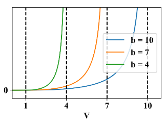
where \(V\) is the volume of the activation maps² and \(b\) is the budget. For this figure, \(a=1\); this hyperparameter corresponds to the value of \(V\) where the budget is comfortably respected. The barrier function is multiplied with the sparsity loss:

During training, \(b\) is transitioned from a value larger than the initial \(V\), to \(B\), the “final budget”.

The complete loss function is the sum of a data term and the sparsity loss term (above). The data term can be a cross-entropy, but a Knowledge Distillation objective is suggested for easier pruning.

Mixed-Connectivity Block

By pruning feature maps in residual blocks, atypical connectivity emerges:

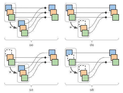
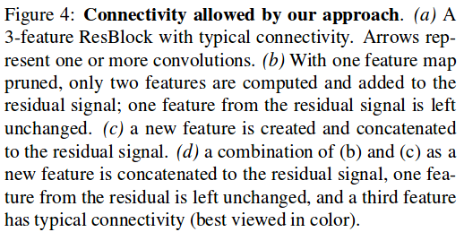
These connectivity patterns generally do not provide computational savings, unless they are leveraged by a special Mixed-Connectivity block implementation (given in the paper).

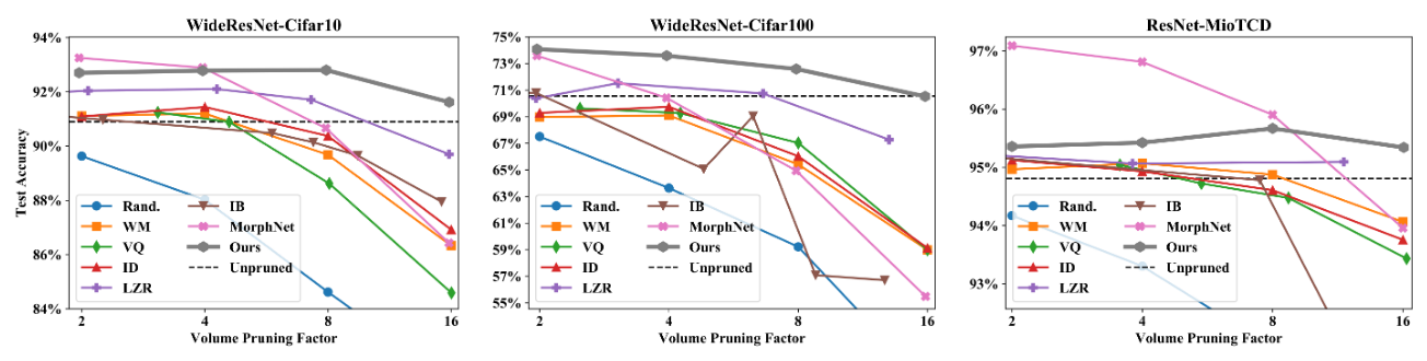
Results

At the highest pruning factors, this method outperforms the state of the art. It also requires less hyperparameter tuning.

---

Notes