On Multiplicative Integration with Recurrent Neural Networks
Main idea
Replace the RNN core additive block with a multiplicative block using the Hadamard product.
[Reminder] Hadamard product: \((A \odot B)_{ij} = a_{ij} \times b_{ij}\)
Core block of Vanilla RNN vs Proposed Multiplicative-Integration RNN (MI-RNN):
 \(\rightarrow\)
In a more general form, where each matrix has its own bias term:
Finally, with an added “gate” on the second order term:

(If \(\alpha = 0\), we get back to the original additive block)
NOTES:
- Number of parameters is about the same
- Second-order term shares parameters with first-order terms
- Can be easily added to existing architectures (e.g. LSTM/GRU)
Gradients
Gradient for vanilla-RNN:
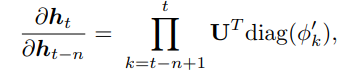
Gradient for MI-RNN:
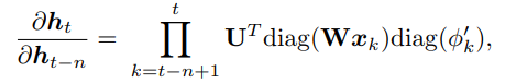
(For the simple case. In the general case, we have: diag\((\alpha \odot W x_k + \beta_1)\))
NOTES:
- Gradient is now “gated” by \(\text{diag}(Wx_k)\)
- Gradient propagation is easier with \(Wx_k\) involved
Experiments using Penn-Treebank (text) dataset
Activations problem
Activations over the validation set, using tanh as the nonlinearity
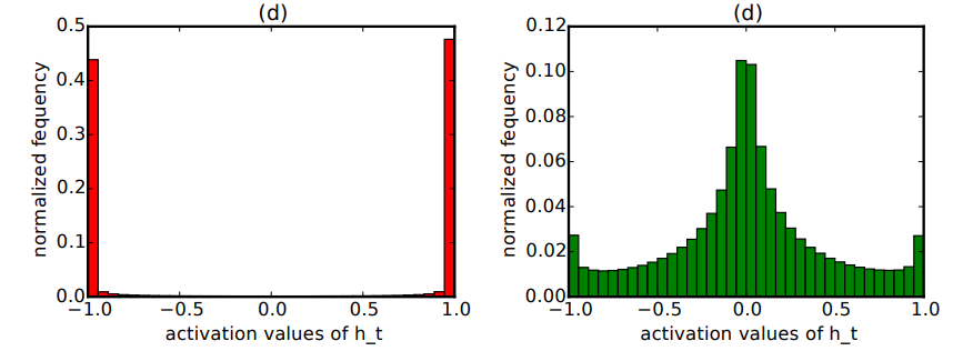
[Reminder] Tanh derivative: \(\nabla \tanh(x) = 1 - \tanh^2(x)\)
- For saturated activations, \(\text{diag}(\phi'_k) \approx 0\) (no gradient flow)
- For non-saturated, \(\text{diag}(\phi'_k) \approx 1\)
Scaling problem
- Pre-activation term : \(Wx_k + Uh_{k-1}\)
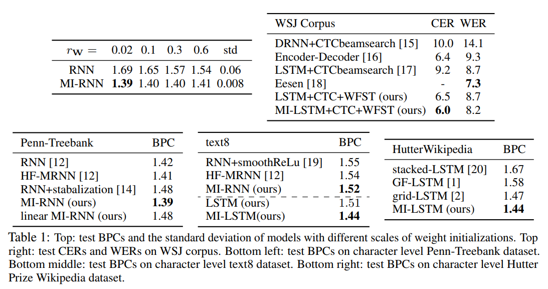
- For one-hot vectors, \(Wx_k\) is much smaller than \(Uh_{k-1}\); initialization matters a lot! (See top-left of Fig.1, where \(r_w\) is the uniform initialization range)
Comparative experiments