HAMLET: Hierarchical Harmonic Filters for Learning Tracts from Diffusion MRI
Contribution
The authors propose a new set of learnable filters for extracting both location and orientation of a specific white matter bundle in the human brain. In that sense, their proposal combines the ideas of bundle specific tracking and pure bundle segmentation.
As opposed to common deep learning approaches, their filter needs only a few parameters to map 12 chosen bundles (1e3 for HAMLET vs 1e6 for common CNN implementations in other tasks).
Further, their approach makes use of covariance properties of the data, i.e. translation as well as rotation covariance.
These two factors enable their filter to be trained with a relatively modest number of training samples.
Overview
Covariant Non-linear filters based on Spherical Tensor Algebra
Prereqisites
-
Spherical tensor fields
\(x(\mathbf{r}, \mathbf{n}) = \sum_{j=0}^\infty \mathbf{a}^j(\mathbf{r})^\mathsf{T} \mathbf{Y}^j(\mathbf{n})\).
- \(\mathbf{Y}^j: S_2 \mapsto \mathbb{C}^{2j+1}\) are SH basis functions of order j.
-
\(\mathbf{a}^j: \mathbb{R}^3 \mapsto \mathbb{C}^{2j+1}\) is a spherical tensor field.
-
Spherical product
The authors define a spherical product \(\circ_j : \mathbb{C}^{2j_1+1} \times \mathbb{C}^{2j_2+1} \mapsto \mathbb{C}^{2j+1}\) which is rotationally covariant in the sense of
\((\mathbf{D}^{j_1}(g)\mathbf{v}) \circ_j (\mathbf{D}^{j_2}(g) \mathbf{w}) = \mathbf{D}^j(g)(\mathbf{v} \circ_j \mathbf{w})\),
where \(\mathbf{v} \in \mathbb{C}^{2j_1+1}\), \(\mathbf{w} \in \mathbb{C}^{2j_2+1}\) and \(g \in SO(3)\) and \(\mathbf{D}^j(g)\) is the Wigner-D matrix.
-
Spherical differential operator
Given the solid harmonics defined by the homogeneous polynomials \(R_m^j(\mathbf{r}) = r^jY^j_m(\mathbf{n})\) (where \(r = |\mathbf{r}|\) and \(\mathbf{n} = \frac{\mathbf{r}}{|\mathbf{r}|}\)), they further define a spherical differential operator
\(\mathbf{\partial}^j := (\partial^j_{-j}, ..., \partial^j_{j})\),
where \(\partial^j_m := R^j_m(\nabla)\) on the basis of spherical products.
The authors emphasise that this “operator can be used to linearly map” spherical tensor fields “onto other” spherical tensor fields “by intertwining spatial neighbourhood information”.
Filter composition
The proposed filters are composed similarly to the layers of a conventional CNN. They feature a linear filter with invariance properties, a non-linear transformation as well as linear combination of several channels.
-
Input
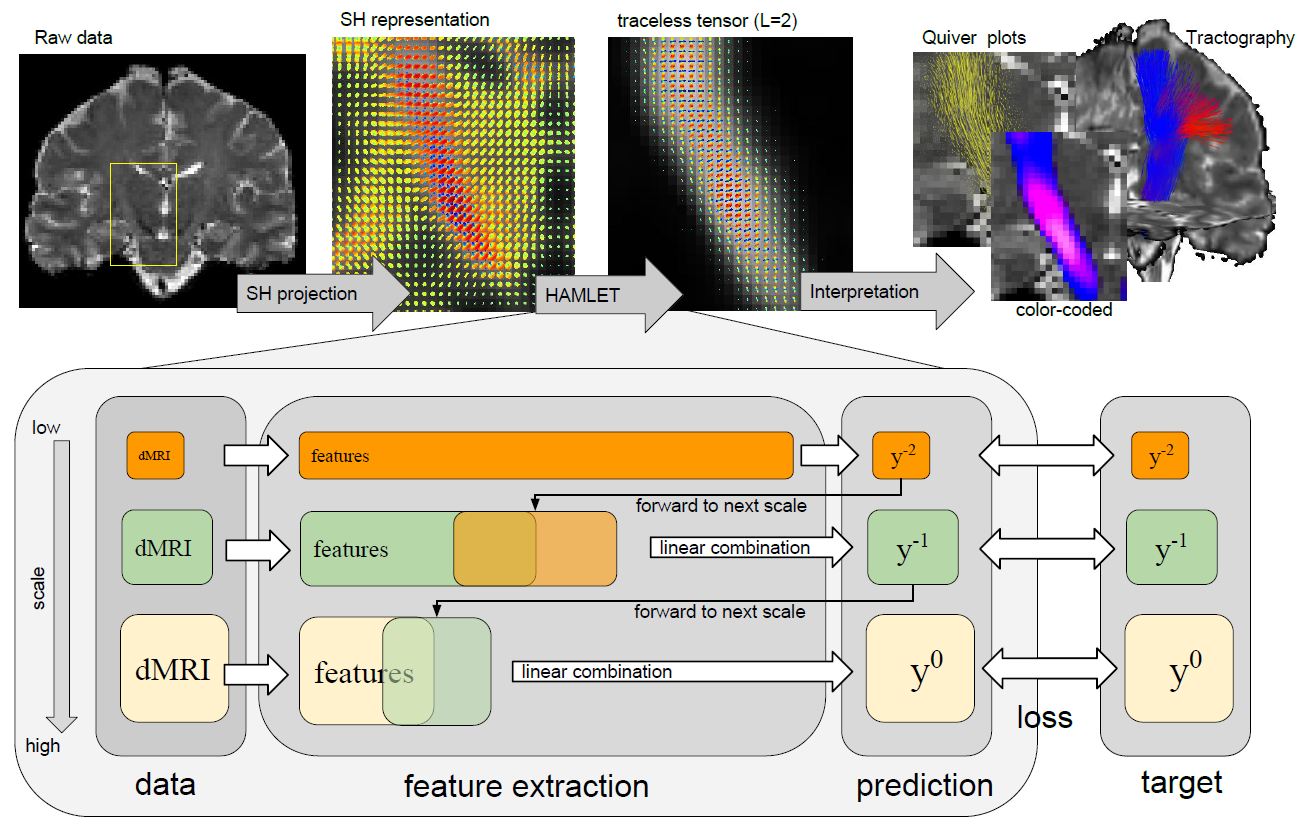
The filters input is composed of the collection of spherical tensor fields given by the expansion of the raw dMRI signal in the spherical harmonics basis. In their experiments, the authors use only order 0th and 2nd order coefficients resulting in
\(D = \{\mathbf{a}^0, \mathbf{a^2}\}\).
-
A. Linear features
The linear features are obtained by convolving the spherical tensor fields with a Gaussian (g) and projecting the result onto the basis defined by \(\partial^L \circ_j g\). These features are given as
\(\mathbf{b}_{J, L, j, g} = \partial^L \circ_J (g \ast \mathbf{a}^j)\).
-
B. Non-linearity and mapping to 2nd order tensor
Subsequently, non-linearity is achieved by considering spherical products of these linear features. Since the authors assume single bundles to be sufficiently represented by 2nd order tensors locally, they map the spherical products back to order two, resulting in the feature maps
\(\mathbf{f}_j(\mathbf{b}_I, \mathbf{b}_{I'}) = \partial^L \circ_2 (g \ast (\mathbf{b}_I \circ_j \mathbf{b}_{I'})\).
-
C. Linear combination of channels
Finally, the features of different channels are linearly combined to obtain the final filter output \(\mathbf{y}\) as
\(\mathbf{y}(D) = \sum_{j, I, I'} \alpha_{jII'} \mathbf{f}_j(\mathbf{b}_I, \mathbf{b}_{I'})\).
Hierarchical composition
Since the filters are applied in a multi-resolution approach (see overview figure above) it is necessary to specify how features are forwarded to subsequent scales.
Given the results on scale s, the filter output on scale \(s+1\) is obtained by
\(\mathbf{y}^{s+1} := \kappa^s\mathbf{y}^s + \vert\mathbf{y}^s\vert \sum_{j,I,I'} \alpha^s_{jII'} \mathbf{f}_j(\mathbf{b}^{s+1}_I, \mathbf{b}^{s+1}_{I'}) + \sum_{j,I,k} \beta^s_{jIk} \mathbf{f}_j(\mathbf{b}^{s+1}_I, \mathbf{y}^s_k)\),
which is composed by
- a. the features \(\mathbf{y}^s\) from the previous scale s
- b. the newly obtained features from scale \(s+1\)
- c. a mixed term of features \(\mathbf{y}^s\) from scale s and new linear features \(\mathbf{b}^{s+1}_I\) from scale \(s+1\).
Training
The parameters \(\kappa, \alpha\) and \(\beta\) are learned during training.
Given the “trace” of a “tract” the authors define their ground truth as the normalised density map. The unnormlised density map is obtained as
\(\mathbf{y}(\mathbf{r}) = \sum_k \int \mathbf{Y}^2(\mathbf{n}(t)) \delta(\mathbf{r}_k(t) - \mathbf{r})\mathrm{d}t\),
where \(\mathbf{r}_k\) is the parameterisation of a “tract” (?) (check paper for details).
Experiments
The experiments are performed on two different data sets. Training is done on a high quality dataset on a Siemens PRISMA scanner (58 directions, b-value \(\in \{1000, 2000}\) for 55 subjects. Testing (and retesting) uses a low quality data set from a TRIO scanner (60 directions, b-value unkown) on 28 subjects in two sessions.
Ground truth tractography is based on global tractography (check paper for more details). The authors choose 12 bundles to evaluate on.
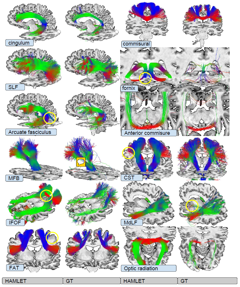
Qualitative assessment on PRISMA test data
Euler integration is used to obtain streamlines from HAMLET output. Thresholding of the output is performed by “optimising the segmentation accuracy”.
The comparison of tractography output for HAMLET and the ground truth a random test subject from the PRISMA data set is used. The authors find their results overall visually appealing. However, they acknowledge artifacts (yellow circles in the figure below) in the results of their own method. One source of error is high variability in the ground truth data which causes their output to have low confidence and therefore the thresholding is more prone to cut away parts of the bundle volume in such regions.
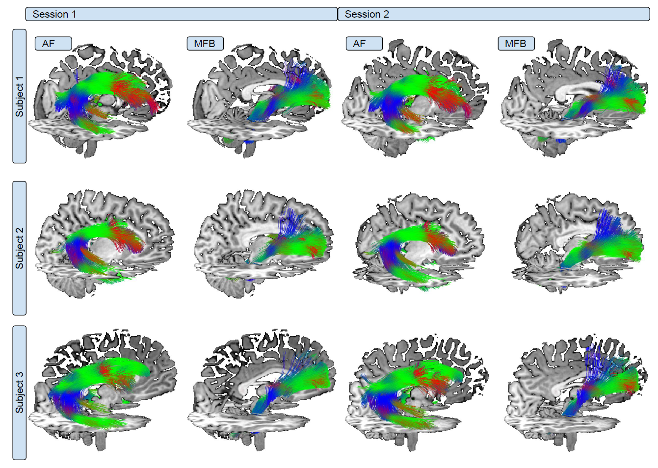
Test-retest and extrapolation to unseen acquisition protocol
In a second experiment they assess HAMLET’s
- a. ability to generalise to different acquisition protocols
- b. robustness to repeated measurements.
The below figure shows test results of three subjects on the TRIO data set for HAMLET after training on PRISMA for the two acquisition time points.
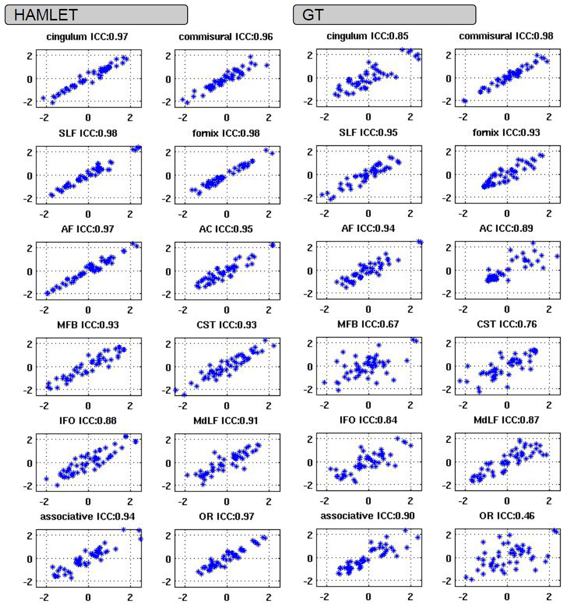
In order to quantify the retest reproducibility, they assess the “apparent tract volume” computed on the output of HAMLET which they define as “the squared power” of the output map y given by
 .
.
Based on the correlation plots in the figure below, the authors aim to show the robustness of that measure (and thus their method) with respect to repeated measurements.