Contribution

The authors present an unsupervised approach for improving the performance of a given CNN by improving its performance for those training samples which are hard to predict.

Main idea

Given a meaningful initial representation (in the following denoted by \(g\)), the authors first identify difficult positive samples as well as difficult negative samples (w.r.t. a fixed anchor sample). Then, during training they try to minimise the distance between anchor and positive sample and to maximise the distance between anchor and negative sample.

Nearest neighbour graph

In order to compute manifold distances the authors employ a Euclidean nearest neighbour graph \(G\). Even though their computations are based on the complete adjacency matrix of \(G\), the authors state that the overall effort is limited thanks to their efficient implementation and the fact that for each anchor sample only k nearest neighbours would have to be computed.

Selection of training samples

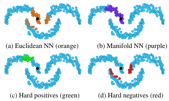
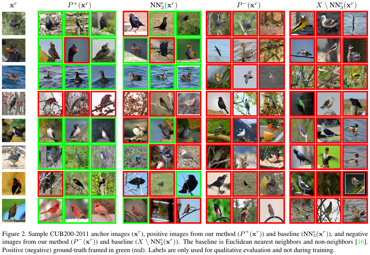
• Positive samples are defined as the set of k-nearest-neighbours in the Euclidean sense subtracted by the set of k-nearest-neighbours on the manifold of the anchor point \(\mathbf{x}^r\) in the given representation space (i.e. \(\mathbf{y}^r = g(\mathbf{x}^r)\) where \(g\) denotes the feature transform):

  \[P^+(\mathbf{x}^r) = \{\mathbf{x} \in X \, : \, g(\mathbf{x}) \in \mathrm{NN}^m_k(\mathbf{y}^r) \backslash \mathrm{NN}^e_k(\mathrm{y}^r)\}\]

• Negative samples are defined in the opposite way:

  \[P^+(\mathbf{x}^r) = \{\mathbf{x} \in X \, : \, g(\mathbf{x}) \in \mathrm{NN}^e_k(\mathbf{y}^r) \backslash \mathrm{NN}^m_k(\mathrm{y}^r)\}\]

• Anchor samples should provide many relevant training samples to improve the manifold and redundancy between their sets of samples should be avoided. The authors choose to compute them as the modes of their nearest neighbour graph \(G\).

Loss functions

Two loss functions are proposed.

• Contrastive loss:

  \[l_c(\mathbf{z}^r, \mathbf{z}^+, \mathbf{z}^-) = ||\mathbf{z}^r - \mathbf{z}^+||^2 + [ m - ||\mathbf{z}^r - \mathbf{z}^-|| ]^2_+\]

• Triplet loss:

  \[l_t(\mathbf{z}^r, \mathbf{z}^+, \mathbf{z}^-) = [ m + ||\mathbf{z}^r - \mathbf{z}^+||^2 - ||\mathbf{z}^r - \mathbf{z}^-||^2 ]_+\]

Experiments

The approach is tested in two scenarios. a. Fine-grained categorization. b. Particular object retrieval. In both it achieves at least state of the art performance. (For results of the second case, check the paper.)

Fine-grained categorization

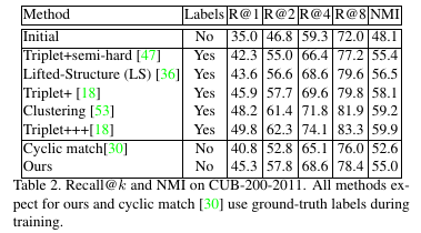
For this experiment, the CUB200-2011 data set with 200 classes is used (100 for training, 100 for testing). The initial representation space is given by the R-MAC features on the last convolutional layer of the pre-trained GoogLeNet (on ImageNet). Triplet loss is employed.

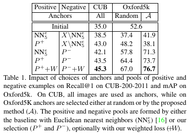
Comparing the impact of their different samplings of training data, the authors found that employing \(P^+\) and \(P^-\) gave best results (even better when weighing the loss with the respective manifold distances).

Comparing with fine-tuned approaches on the given data set, the proposed method achieves comparable performance. Note, that most methods to compare to are not unsupervised.