Tensor-Train Recurrent Neural Networks for Video Classification
Problem
Classifying videos with deep learning architectures is hard
CNN only
Two options:
- Big 3D volumes with variable sizes that might not fit into memory.
- Process each frame separately and fuse the results to make a prediction
CNN+RNN
Using CNN+RNN with end-to-end training is impractical. In practice, 2 options were explored :
- Focus on the CNN part and reduce the sequence length
- Focus on the RNN part and use a pre-trained CNN (no end-to-end training)
RNN only
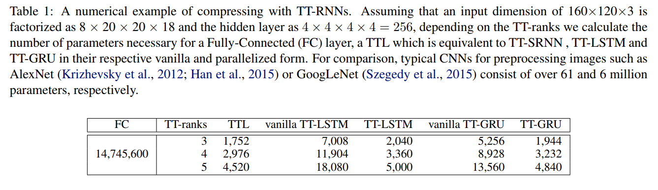
Using only an RNN is also a problem, given the input dimensionality (e.g. a video with \(160 \times 120 \times 3\) frames results in a \(57,600\) input vector, and \(5,760,000\) parameters if using a 100-units hidden layer).
Summary
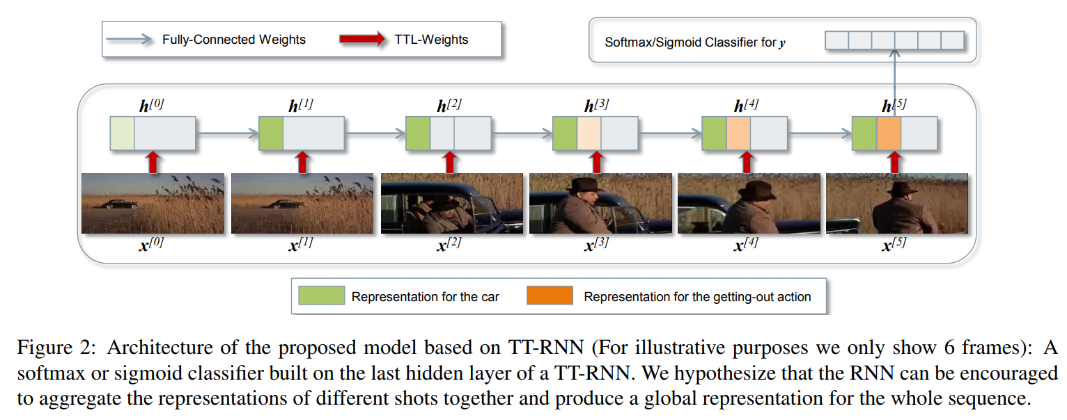
The paper focuses on RNN-only video classification using raw pixels. To reduce the input dimensionality, the input-to-hidden matrix is factorized with the Tensor-Train decomposition.
Tensor-Train Factorization
Step 1: Factorization
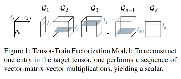
Each entry in the target tensor is represented as a sequence of matrix multiplications using elements selected from core-tensors.
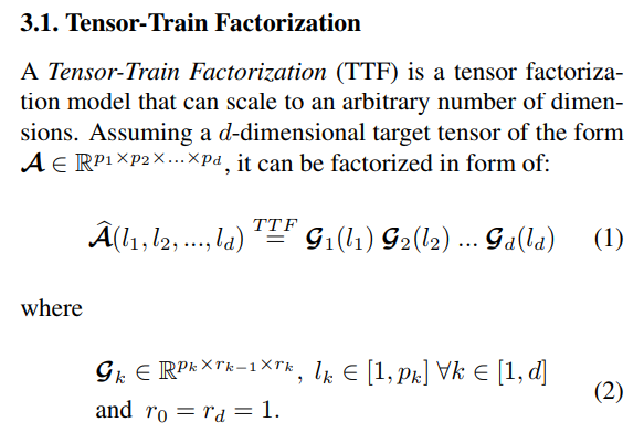
Each index \(l_k\) is used to select an element from the core-tensors along the first dimension \(p_k\). Note that since \(r_0 = r_d = 1\), the result is always a scalar.
Visually :
Step 2: Preliminary steps for Feed-Forward layer factorization
We add the constraint that each integer \(p_k\) can be factorized as \(p_k = m_k \cdot n_k \, \forall \, k \in [1,d]\). Then, we reshape \(\mathcal{G}_k\) into \(\mathcal{G}_k^* \in \mathbb{R}^{m_k \times n_k \times r_{k-1} \times r_k}\). Each index \(l_k\) can be uniquely represented with two indices \((i_k, j_k)\):
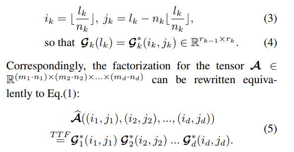
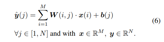
Step 3: Feed-Forward Layer Factorization
The usual notation for a feed-forward layer is: \(\hat{\mathbf{y}} = \mathbf{Wx} + \mathbf{b}\) The equation is rewritten in an equivalent way using scalars:
If both \(M\) and \(N\) can be factorized into integer arrays of length \(d\), i.e. \(M = \prod_{k=1}^d m_k, N = \prod_{k=1}^d n_k\), then \(\mathbf{x}\) and \(\hat{\mathbf{y}}\) can be reshaped to have the same number of dimension: \(\mathcal{X} \in \mathbb{R}^{m_1 \times ... \times m_d}\), \(\mathcal{Y} \in \mathbb{R}^{n_1 \times ... \times n_d}\). The mapping function \(\mathbb{R}^{m_1 \times ... \times m_d} \rightarrow \mathbb{R}^{n_1 \times ... \times n_d}\) is rewritten as:
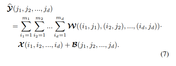
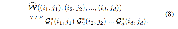
Thus, Eq.6 is a special case of Eq.7 with \(d = 1\). Finally, the weight tensor \(\mathcal{W}\) can be replaced by the TTF representation:
Step 4: Tensor-Train RNN
The LSTM has 4 “gates”, or weights matrices. Each of those matrices can have a TTF representation. However, a concatenation trick can be used like most LSTM implementations. Thus, all gates are concatenated as one big output tensor which can be compressed even more.
Experiments
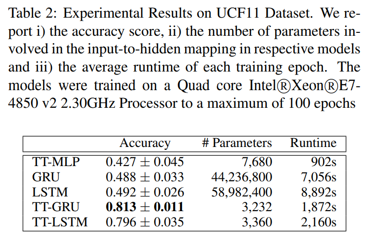
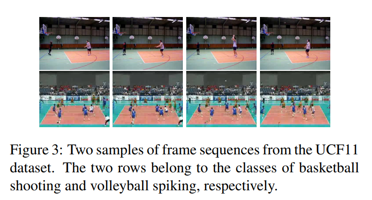
UCF11 (Youtube Action Dataset)
- 1600 video clips
- 11 classes
- \(320 \times 240\) downsampled to \(160 \times 120\), at 24 fps
- Sequence length varies between 204 and 1492
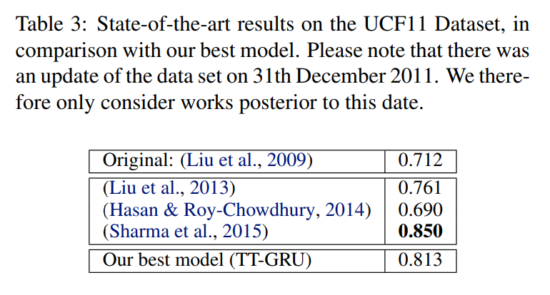
- (Liu et al., 2013): SIFT/STIP + Harris3D Corner Detector + Optical Flow + GMM w/ EM
- (Hasan & Roy-Chowdhury, 2014): Ensemble of multi-class SVMs
- (Sharma et al., 2015): Pre-trained GoogLeNet CNN + 3-fold stacked LSTM + Attention
Training times: 8-10 days for GRU/LSTM vs. 2 days fro TT versions.
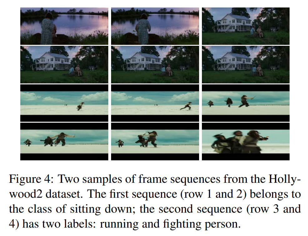
Hollywood2 Data
- 69 movies (33 training, 36 test) -> 823 training clips, 884 test clips
- 12 labels, multiclass
- \(234 \times 100\), at 12 fps
- Sequence length varies between 29 and 1079
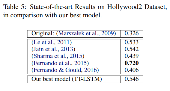
- (Sharma et al., 2015): Pre-trained GoogLeNet CNN + 3-fold stacked LSTM + Attention
- (Fernando et al., 2015): Frame features + Frame ordering -> Learned representation -> SVM classifier
- (Fernando & Gould, 2016): Frame-wise CNN + “Rank pooling” + Softmax