Ship wake-detection procedure using conjugate gradient trained artificial neural networks
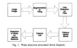
This paper developed a method to reduce large two-dimensional images to significantly smaller “feature lists.” These feature lists overcome the problem of storing and manipulating large amounts of data.
A new artificial neural network using conjugate gradient training methods was successfully trained to determine the presence or absence of wakes in radar images.
Images: radar, 4000 x 4000 pixels for a 25m of resolution by pixel
Because radar satellite frame rate is less than a frame per second and their image resolution is low, it is hard to get ocean-surface features. However, the internal wave signature due to tidal flows over the continental shelf and ship wakes were observed in Seasat data. These activities have a long duration and allow ship detection.
In order to ensure that the entire wake appears in the digital representation, radar images would require between 10^6 and 10^8 pixels.
Main Idea
A wake-detection system based on techniques for mapping input radar images into sets of one-dimensional feature lists, which can then be input to an artificial neural network. The mapping significantly reduces the quantity of data, which reduces the memory and training requirements so that an artificial neural network can be used.
Results are presented for a wake-processing system operating on radar imagery produced by numerical simulation and by data collected with the NASA-JPL AirSAR. They show that a new conjugate gradient training can be possible.
A new conjugate gradient training method is applied to back-propagation learning showing better results that the conventional steepest-descent method.
Preprocessing
They use concepts of plane-wave detection in the Fourier space to develop the algorithm.
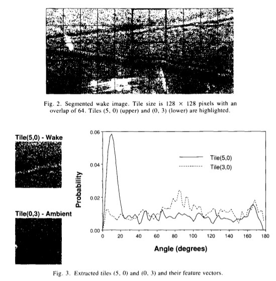
“Line detection” is the Fourier transform of a function \(f(x,y)\) with the Fourier power spectrum by \(\|F\|^{2} = FF*\).
“feature vector” is the normalization of the signal to its sum.
“Feature list” is a pair of numbers, one for each tile, consisting of the maximum probability and its angle.
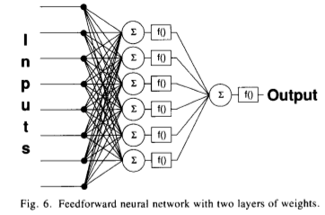
Network
Summary:
-
A starting \(\vec{x}_{\,0}\) point is selected by initializing the weights randomly, uniformly distributed between -0.5 and +0.5. The gradient \(\vec{g}_{\,0}\) is computed at this point and an initial search direction vector \(\vec{d}_{\,0}=-\vec{g}_{\,0}\) is selected.
-
The constant ak which minimizes \(f(\vec{x}_{\,k}+\alpha_{\,k}\vec{d}_{\,k})\) is computed by line search. The weight vector is updated to the new point: \(\vec{x}_{\,k+1}=\vec{x}_{\,k}+\alpha_{\,k}\vec{d}_{\,k}\).
-
The termination criteria are evaluated at the new point. If the error at this point is acceptable or if the maximum number of function and gradient calculations has been reached, the algorithm terminates.
-
A new direction vector \(\vec{d}_{\,k+1}\) is computed. If \(k+1\) is an integral multiple of \(N\) (the dimension of \(\vec{x}\)), then \(\vec{d}_{\,k+1} = -\vec{g}_{\,k+1}\). Otherwise, \(\vec{d}_{\,k+1} = -\vec{g}_{\,k+1}+\beta_{\,k}\vec{d}_{\,k}\), where \(\beta_{\,k}\) is computed according to the method selected by the user: Fletcher-Reeves, Polak-Ribikre, or Hestenes-Stiefel.
-
\(k\) is replaced by \(k + 1\) , and the algorithm continues as before in Step 2.
To augment the number of images, they created a simulator to generate synthetic feature lists, since they have only a limited number of SAR images. They generated feature lists for wakes oriented at 0” and 180”, with arm angles varying between 0” and 20” (a 0 arm angle simulated a wake in which one of the arms was obscured), over a range of variances. The training set consists of 232 simulated feature lists(wake), of which half are ambient(no wake). The network was trained using the simulated feature lists only and tested on real data. The feature lists were presented to the network in the form of one-dimensional data, interleaving probability with an angle.
Results
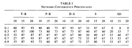
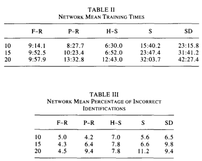
They use the following five methods in their neural network implementation: Fletcher-Reeves, Polak-Ribière, Hestenes-Stiefel, Shanno, and steepest descent. The learning parameters (convergence parameters), are 0.1, 0.3, 0.5, 0.7, and 0.9.