Convolutional Recurrent Neural Networks for Hyperspectral Data Classification

Description

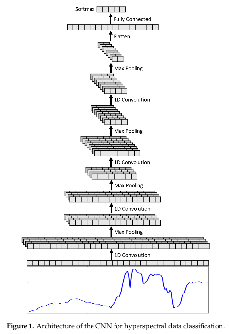
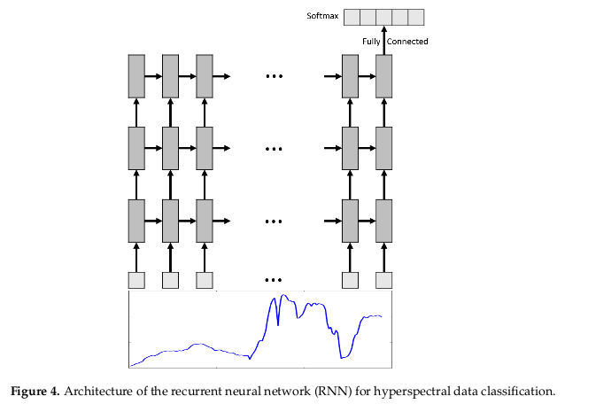
One-dimensional CNNs are already used to extract spectral features for hyperspectral data in some papers¹. Two-dimensional CNNs have been employed to extract features for hyperspectral data in others. CNNs can also be used for scene classification of high-resolution remote sensing RGB images. In a paper of 2016, an RNN was used for land cover change detection on multi-spectral images.

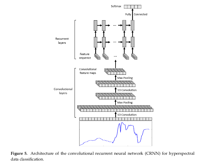
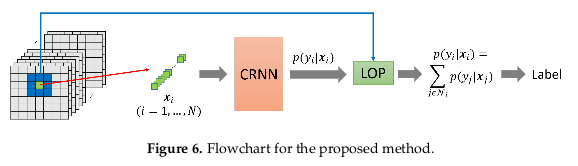
So the idea in this paper is to combine the best of the RNN with a CNN, to be able to make a better spatial classification with all the spectral information available. The CRNN is a hybrid of convolutional and recurrent neural networks. It is composed of several convolutional (and pooling) layers followed by a few recurrent layers (Figure 5). First, the convolutional layers are able to extract middle-level, abstract and locally invariant features from the input sequence. The pooling layers help reduce computation and control overfitting. Then, the recurrent layers extract contextual information from the feature sequence generated by the previous convolutional layers. Contextual information captures the dependencies between different bands in the hyperspectral sequence.

For the CNN input, they give the spectral information, which passes in 1D convolutions and max pooling and the result of those convolutional layers is the input sequence for the RNN.

To improve the pixel classification operation, because the neural networks will preserve the spectral features for each pixel independently, the authors add a linear opinion pools (LOP) in the system²³. The LOP-based decision fusion is a probability for each pixel \(x_i\) as a weighted sum of the posterior probabilities of the spatial neighbors of that pixel.

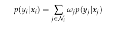
Where \(N_i\) are the spatial neighbors of pixel \(x_i\) and \(w_j\)’s are weights for each neighbor.

That method improves the classification by smoothing out noisy predictions and help to classify based on spatially neighboring pixels, knowing then neighbors tend to have similar categories.

DataSets

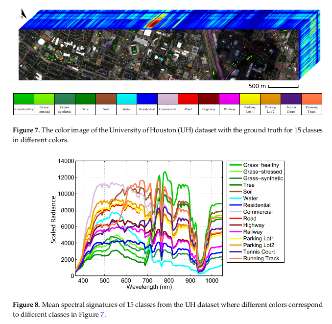
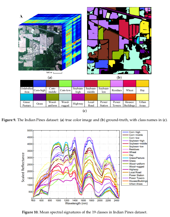
The University of Houston (UH) hyperspectral image (144 bands).

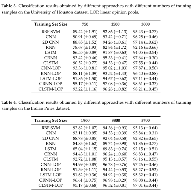
Indian Pines (180 bands).

Results

To verify the accuracy, they wanted to know if the number of samples will change a lot the average accuracy. So they use 50, 100 and 200 samples for the Houston University dataset and 100, 200 and 300 samples for each class for the Indian Pines dataset.

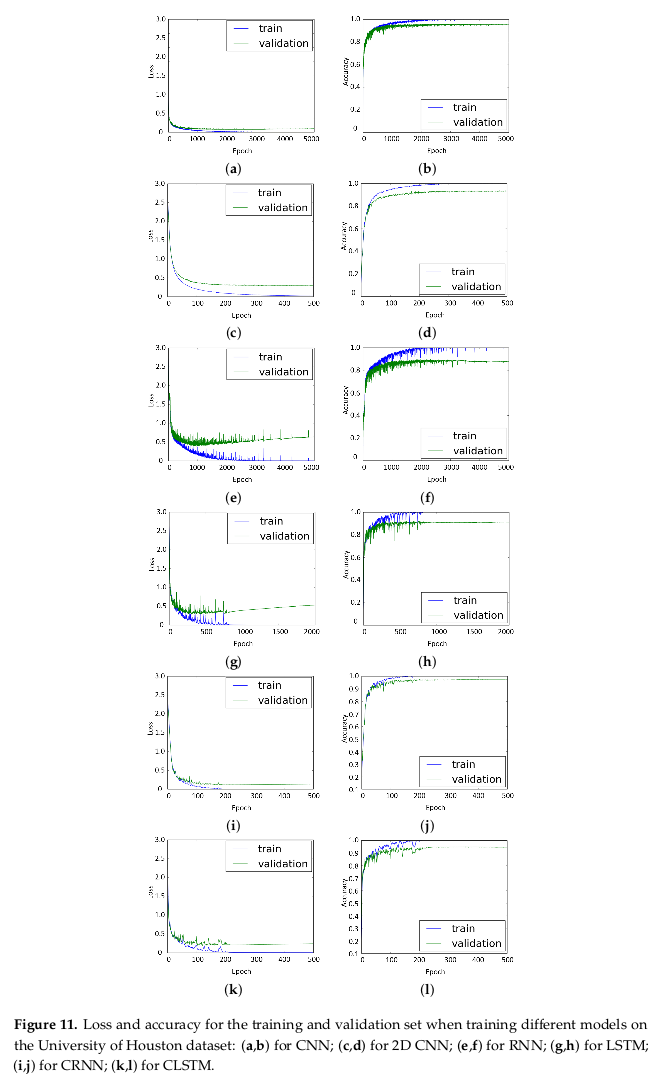
At the same time, the validation losses all converged to a low level, and the validation accuracies all reached a high number with a very low noise.

Strong points

• Recurrent layers can handle variable-length input sequences.
• The small number of images needed.
• Easy to understand the extracted information in the convolutional layers.

In the future

They want to explore the semi-supervised deep learning techniques for hyperspectral image classification.