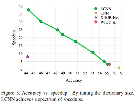
LCNN is a novel layer that can replace any convolutional layer. The main thing is that a filter is “decomposed” as a linear combination of parts from a dictionary. The ability to tune the dictionary size and the number of elements in the linear combination allows an efficiency/accuracy trade-off (see Figure 3). In addition, the authors argue that LCNN has an advantage in few-shot learning and few-iteration learning settings.

Filter Construction

Let’s first define the 4 tensors that we’ll need:

• \(\bold{W} \in \mathbb{R}^{m \times k_w \times k_h}\) is a filter, where \((k_w, k_h)\) are its spatial dimensions and \(m\) is the number of channels in the input image.
• \(\bold{D} \in \mathbb{R}^{k \times m}\) is the dictionary. It contains \(k\) vectors of size \(m\). Those vectors will be combined to construct the filter (See Figure 1).
• \(\bold{I} \in \mathbb{N}^{s \times k_w \times k_h}\) is the lookup indices tensor, where \(s\) is the number of elements in the linear combination.
• \(\bold{C} \in \mathbb{R}^{s \times k_w \times k_h}\) is the coefficient tensor.

Then, we can formulate the construction as follows:

\[\bold{W}_{[:,r,c]} = \sum_{t=1}^s \bold{C}_{[t,r,c]} \cdot \bold{D}_{[\bold{I}_{[t,r,c]},:]}\]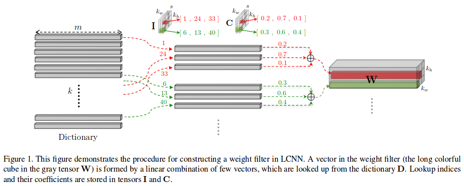

Fast Convolution using a Shared Dictionary

Now, let’s imagine that our dictionary is in fact the weights of a 1x1 convolution layer: we thus have \(k\) filters of dimensions \((m, 1, 1)\). By passing our input image \(\bold{X} \in \mathbb{R}^{m \times w \times h}\) through this 1x1 convolutional layer, we get \(\bold{S} \in \mathbb{R}^{k \times w \times h}\). With \(\bold{I}\) and \(\bold{C}\) in hand, we can compute the result of the convolution \(\bold{X} * \bold{W}\) for each filter, without really constructing any \(\bold{W}\). (See section 3.1.1 of paper.) By reducing \(k\) and \(s\), we can reduce the number of lookups and floating point operations.

One problem arises from using indices to select values in tensors: it makes the network non-differentiable. During training, a trick is used to be able to backpropagate. For each filter \(\bold{W}\), a sparse tensor \(\bold{P} \in \mathbb{R}^{k \times k_w \times k_h}\) is constructed. In this tensor, elements at indices \(\bold{I}\) have values \(\bold{C}\). Then, we have that \(\bold{X} * \bold{W} = \bold{S} * \bold{P}\) for each \(\bold{W}, \bold{P}\) pair.

During training, we learn \(\bold{D}\) and \(\bold{P}\). To obtain a tensor \(\bold{P}\) that is \(s\)-sparse, we impose a \(\ell_1\) norm and keep only \(s\) non-zero elements. From \(\bold{P}\), we can easily obtain \(\bold{I}\) and \(\bold{C}\).

Few-shot learning

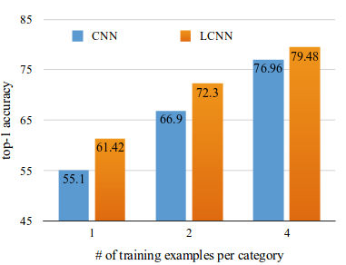
The authors argue that this layer architecture has a performance advantage in few-shot learning settings, as we can see in the following plot (extracted from Figure 4).

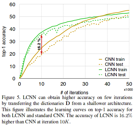
Few-iteration learning

The authors also argue that LCNN can learn more in the first iterations of training than an ordinary CNN. In one experiment, they transferred the dictionary learned with a shallow network to a deeper network and only trained \(\bold{I}\) and \(\bold{C}\). See Figure 5 for the learning curves.