DenseNet : Densely Connected Convolutional Networks
DenseNet is a CNN architecture that includes dense blocks. In a dense block, each layer has access to the feature maps of all preceding layers. Figure 1 shows a dense block.
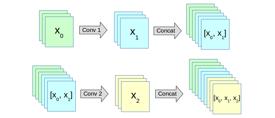
Figure 1: A simplified dense block with two convolutional layers. The block takes \(x_0\) as input and gives \([x_0,x_1,x_2]\) as output. Here, each \(x_i\) is a set of three feature maps. We can see that \(x_0\) is used to produce \(x_1\), and reused to produce \(x_2\).
DenseNets have many advantages :
- They require substantially fewer parameters and less computation to achieve state-of-the-art performances;
- They naturally integrate the properties of identity mappings and deep supervision;
- They are very compact, since they allow feature reuse.
Architecture
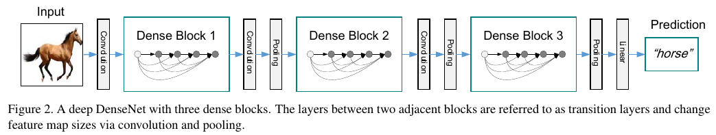
Dense blocks are chained together using transition layers. The transition layers have the purpose of reducing the spatial extents of their inputs, and can also “compress” the feature maps to a smaller number. Figure 2 shows an example DenseNet architecture.
Results
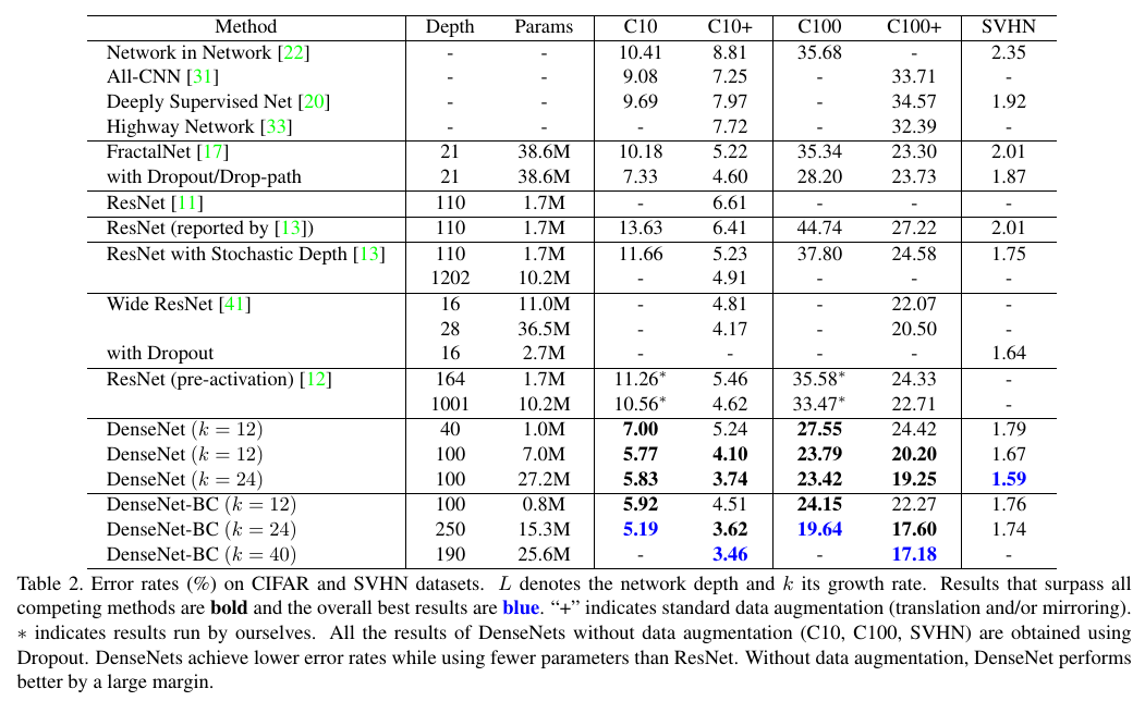
Different DenseNet architecture have stolen the state of the art from FractalNet and Wide ResNet for CIFAR-10, CIFAR-100 and Street View House Numbers. Moreover, DenseNets are on par with ResNets on the ImageNet classification task, using half the number of parameters (see section 4.4 for details).
Efficiency on CIFAR-10
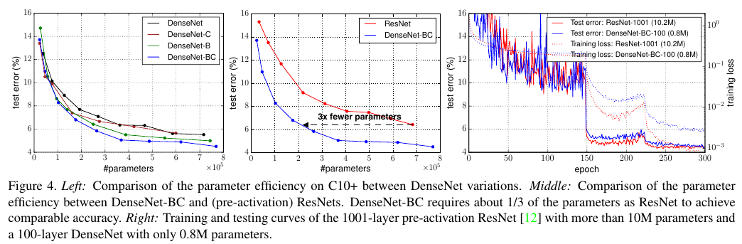
As you can see in the following figure, DenseNets have impressive parameter efficiency and computation efficiency. On the right, see the training and testing curves of a ResNet with 10.2M parameters and a DenseNet with only 0.8M parameters.
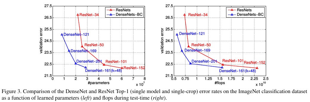
Efficiency on ImageNet
As with CIFAR-10, DenseNets are very efficient for the ImageNet classification task.
Feature Reuse
A very important aspect of DenseNets is feature reuse inside dense blocks. To prove this, the authors made an experiment. The goal was to observe if the connections to early layers in a block are really important. After having trained a DenseNet, they have plotted (see below) the strength of the connections from a layer to all previous layers.
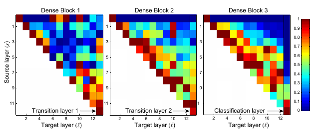
Figure 5: Strength of the connections from a layer \(l\) to a source layer \(s\). The first row represents the connections from all layers to the input of the block. The last column represents the connections from the transition layer to all layers in the block.