Batch Normalization (BN) is a layer to be inserted in a deep neural network, to accelerate training.¹

Why use it

We want to reduce Internal Covariate Shift, the change in the distributions of internal nodes of a deep network during training. It is advantageous for the distribution of a layer input to remain fixed over time. To do so, we will fix the means and variances of layer inputs.

Consider a layer with sigmoid activation \(z = g(Wu + b)\). For all dimensions of \(x = Wu + b\) except those with small absolute values, the gradient flowing down to \(u\) will vanish and the model will train slowly. Since \(x\) is affected by \(W, b\) and the parameters of the layers below, changes to those parameters during training will likely move many dimensions of \(x\) into the saturated regime of the sigmoid and slow down training.

Training converges faster when the inputs of the network are whitened (linearly transformed to have \(\mu = 0, \sigma^2 = 1\), and decorrelated). Thus, we’d like to apply whitening to the input of each layer.

How it works

Normalize each feature independently. Consider a layer with \(d\)-dimensional input \(\bold{x} = (x^{(1)} \ldots x^{(d)})\). We normalize each dimension \(k\) like so :

\[\hat{x}^{(k)} = \frac{x^{(k)} - \mathrm{E}[x^{(k)}]}{\sqrt{\mathrm{Var}[x^{(k)}]}}\]

where the mean and variance are computed on the mini-batch.

Add an affine transform just after. Only applying a normalization can reduce the representational power of the network. For example, a sigmoid would be constrained to its linear regime. Following the normalization by a learnable affine transform addresses this issue. The BN operation becomes :

\[y^{(k)} = \gamma^{(k)}\hat{x}^{(k)} + \beta^{(k)}\]

Notice that if the parameters would learn the values \(\gamma^{(k)} = \sqrt{\mathrm{Var}[x^{(k)}]}\) and \(\beta^{(k)} = \mathrm{E}[x^{(k)}]\), we would recover the original activations, if that were the optimal thing to do.

Constant normalization during inference. During inference, we want the output to depend only on its input (not on other examples). For this, instead of the mini-batch statistics, we use statistics from the whole population, which are constant. In practice, we compute these statistics during training using moving averages. Since the normalization is now fixed, it can be composed with the scaling by \(\gamma\) and shift by \(\beta\), to yield a single linear transform.

Why do we need to backprop through it ? Consider a layer \(x = u + b\), where \(b\) is a learned bias. We normalize the result using the mean of the activation computed over the whole training data : \(\hat{x} = x - \mathrm{E}[x]\). If a gradient descent step ignores the dependence of \(\mathrm{E}[x]\) on \(b\), then it will update \(b \leftarrow b + \Delta b\), where \(\Delta b \propto \partial \text{loss} / \partial \hat{x}\). Then,

\[u + (b + \Delta b) - \mathrm{E}[u + (b + \Delta b)] = u + b - \mathrm{E}[u + b]\]

thus the normalization canceled the effect of the update of \(b\). As training continues, \(b\) will grow indefinitely while the loss remains constant. To address this, we must view the normalization as a transformation taking both the sample \(x\) and the whole mini-batch \(\mathcal{X}\) :

\[\hat{x} = \mathrm{Norm}(x, \mathcal{X})\]

This means that we need to compute two Jacobians :

\[\frac{\partial \mathrm{Norm}(x, \mathcal{X})}{\partial x} \qquad \frac{\partial \mathrm{Norm}(x, \mathcal{X})}{\partial \mathcal{X}}\]

The latter term allows us to consider the mini-batch statistics in the process of gradient descent, which in turn avoids the parameter explosion described above.

How to use it

Put BN before nonlinearities. Since the input \(u\) of an affine layer \(x = Wu + b\) is likely the output of another nonlinearity, the shape of its distribution is likely to change during training, and constraining its first and second moments would not eliminate the covariate shift. Thus, we normalize \(x\), not \(u\).

Note that since we normalize \(Wu + b\), the bias \(b\) will be canceled by the mean subtraction. Thus, we replace \(z = g(Wu + b)\) by \(z = g(\mathrm{BN}(Wu))\), and the role of \(b\) will be played by \(\beta\).

Interestingly, with BN, back-propagation through a layer is unaffected by the scale of its parameters :

\[\mathrm{BN}((aW)u) = \mathrm{BN}(Wu)\] \[\frac{\partial \mathrm{BN}((aW)u)}{\partial u} = \frac{\partial \mathrm{BN}(Wu)}{\partial u}\] \[\frac{\partial \mathrm{BN}((aW)u)}{\partial (aW)} = \frac{1}{a} \cdot \frac{\partial \mathrm{BN}(Wu)}{\partial W}\]

As seen above, larger weights even lead to smaller gradients.

Adapt the learning process. Simply adding BN layers to a network does not take full advantage of the method. These further steps should be taken :

• Increase learning rate ;
• Remove Dropout, since BN is already a strong regularization ;
• Reduce the \(L_2\) weight regularization ;
• Accelerate the learning rate decay (since the network will train faster) ;
• Remove Local Response Normalization ;
• Shuffle training examples more thoroughly, so mini-batches are better representations of the whole population ;
• Reduce the photometric distortions (data augmentation). Since the network needs less iterations to converge, it will see less examples ; we should thus focus on “real” examples.

What to expect

The following are the results of the experiments shown in the paper.

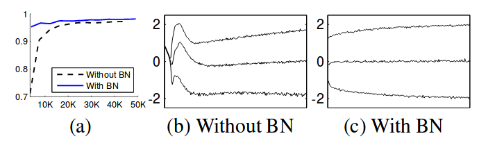
Figure 1 : Results on MNIST using 3 fully-connected hidden layers with 100 neurons each and sigmoid nonlinearity. (a) The test accuracy with and without BN (the x axis is the number of training steps). (b, c) The evolution of input distributions to a typical sigmoid over the course of training. The 15th, 50th and 85th percentiles are shown.

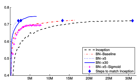
Figure 2 : Results on ImageNet using a variant of Inception (see paper for architecture details – referred to as Inception in the figure). Below are the other architecture variants tested :

• BN-Baseline is Inception with BN before each nonlinearity.
• BN-x5 is Inception with BN and the modifications suggested in the previous section. The learning rate is increased by a factor of 5. The same increase on the original Inception blew up the model.
• BN-x30 is BN-x5 with an initial learning rate 30 times that of Inception.
• BN-x5-Sigmoid is BN-x5 with sigmoid nonlinearity. Training the original Inception with sigmoid nonlinearities was attempted, but the accuracy remained equivalent to chance.

---